Microelectronics, neurophysiology and machine learning, shake up, but do not mix
In the middle of 2018, work on the electrophysiology of the brain of rats was published , with which one unique data set was made publicly available . The dataset is unique in that it contains simultaneous recordings of the local field potential with the help of a new high-density Neuropixels electrode (sample or probe) and a patch electrode from a cell located near the sample. Interest in such records is not only fundamental, but also applied, because it allows validating models for the analysis of neuronal activity recorded by modern samples. And this, in turn, directly concerns the development of new neuroprostheses. What is the principal novelty, and why this dataset is so important - I will tell under the cut.
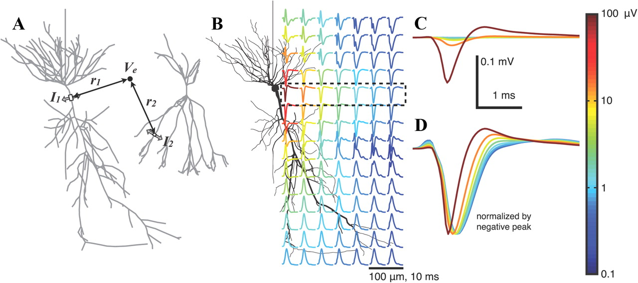
KDPV: the result of modeling the extracellular potential near one neuron in the generation of action potential ( source ). The color indicates the amplitude of the potential. This illustration will be important for further understanding.
Electrophysiological research methodsbrain based on the recording of the electrical potential of the brain. They can be divided into non-invasive - mainly electroencephalography (EEG), and invasive, for example, electrocorticography (ECOG, ECoG), patch clamp (patch-clamp) or registration of local field potential (BOB = local field potentials, LFP) . For the latter, a small electrode with a size of 10-100 μm is injected directly into the brain and its potential is recorded. In order to investigate the mammalian brain activity at the cellular level, i.e., to measure the activity of individual cells, the available non-invasive methods cannot be applied, because the potential from one cell decays in space very quickly, literally over 100 microns (see KDPV). Therefore, in any animal model, as in man,
But with invasive methods is not so simple. To record the activity of a neuron, it is necessary to bring the electrode very close to the neuron, ideally place it inside the cell, as is done in the patch clamp, or with the help of Sharp electrodesthat in practice is difficult, very difficult. On the other hand, any extracellular electrode with a size of ~ 10 μm will register action potentials from 5-10 cells around due to high density of neurons and high ionic conductivity of the extracellular solution. Therefore, the task of registering individual cells is technically resolved by increasing the density of electrodes in the vicinity of the cell. In this regard, modern electrophysiology is moving in the direction of increasing the density of the electrodes, increasing their number and reducing the size. Even among the requirements, there is a need to amplify the signal closer to the registration site, in order to reduce noise, and place a multiplexer to reduce its size. So, in 2016 it was announced in the preprint, and in 2017 it was published in Nature, and in 2018 it was already on the market, a new high-density sample Neuropixels, made by CMOS technology, on 960 electrodes, of which any 384 are available for simultaneous recording. The size of one registration site is 12 microns. The sample thickness is 24 microns. Moreover, with high-density electrodes, as well as with active amplification, people began to work a long time ago, but Neuropixels was the first to reach production and sales, therefore, in the near future, this test will be encountered more and more often in articles.

Fig. Neuropixels scheme. 960 sites are located on a monolithic silicon substrate, as well as a full-fledged multiplexer and an AD interface with 384 channels.
In addition to the classic activity rhythms (alpha, beta, gamma, etc.) responsible for group synchronization, the data obtained using similar samples also contain the action potentials of individual cells (PD = action potentials, AP, spikes, spikes) , which on the record look like short peaks with a duration of ~ 1 ms.
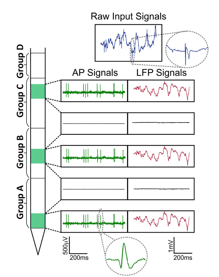
Fig. Signals Neuropixels. Two parts of the signal are distinguished: local field potential (LFP, up to ~ 300 Hz) and cellular activity (AP, from 300 Hz).
Moreover, if the low-frequency local field potential is usually analyzed within the framework of oscillations and spectral or wavelet analysis is used as in the EEG, then the cellular activity contains the action potentials of individual cells, it consists of discrete events against the background of noise. The task of isolating the activity of individual cells is formally reduced to the cocktail party problem, when it is necessary to select a separate speaker from a multitude of speakers. Big data appears when we evaluate the data stream from one such sample. For the analysis of spikes, sampling is carried out at 30–40 kHz with digitization from 16 bits per point (uint16), thus, recording already 100 electrodes for 1 second will weigh from 8 MB. At the same time, experiments usually last hours, which amounts to hundreds of gigabytes from just one working day, and for a full-fledged study you need, say, from 10 such records. Therefore, the potential of this sample also strongly depends on the machine learning algorithms that are used for data analysis.
A typical pipeline for analyzing cellular activity consists of preprocessing, segmentation of spikes and clustering. This part of the research is usually referred to as cluster analysis or spike sorting. Low frequency filtering (> 300 Hz) is usually used as preprocessing, because it is considered that there are no other physiological rhythms above 300 Hz, and only information about individual cellular activity remains. Also during preprocessing in dense samples, it is possible to reduce correlated noise, for example, 50 Hz interference. Segmentation is often taken as a simple threshold, for example, everything above 5 standard deviations of noise can be considered an event. It happens that two-threshold segmentation is used, with a soft and hard threshold, to highlight related events in space and time, as in the watershed algorithm (watershed segmentation ), only in clustering spikes does the distribution of markers take into account the sample topology. After segmentation, a window with a duration of 1-2 ms is taken near the center of each event, and the signal in this window, collected from all channels, becomes a sample for further clustering. This sample is called a spike waveform. Different cells and their different distances from the registration site lead to the fact that their waveforms will differ (see CDRV). As the waveform clustering algorithm itself, EM, template match (template match), deep learning and many variations are used ( topic on github). The only requirement is learning without a teacher. But there is one problem. No one knows for sure what parameters you need to take for your pipeline to make the analysis most effective. Usually, after clustering, the analyst manually passes through the results and makes changes at discretion. Thus, the analysis results can include both algorithm errors and human errors. And they may not be, therefore the question of objective validation remains open.
Validating pipeline can be in several ways. First, changing the external conditions for the object of study. For example, during the experiment, if you study the visual cortex, then you can change the texture, color, brightness of the image. If there is a cell in the analysis that changes its activity depending on the stimulus, then you are lucky. Secondly, you can pharmacologically enhance or reduce the activity of a particular cell type, for example, using blockers of certain channels. Then the activity of your cell will increase / decrease, and you will see the difference in clustering. However, this modulation of activity will also lead to changes in waveforms, because the profile of the action potential over time is completely determined by the kinetics of ion channels. Thirdly, you can optogenetically or using a patch pipette, as in this dataset, measure or induce the activity of certain cells. Due to the large signal-to-noise ratio and the stability of the patch electrode, you will be completely confident in the activity of a single cell. Conceptually, the publication was devoted to assembling a validating dataset using a patch clamp.
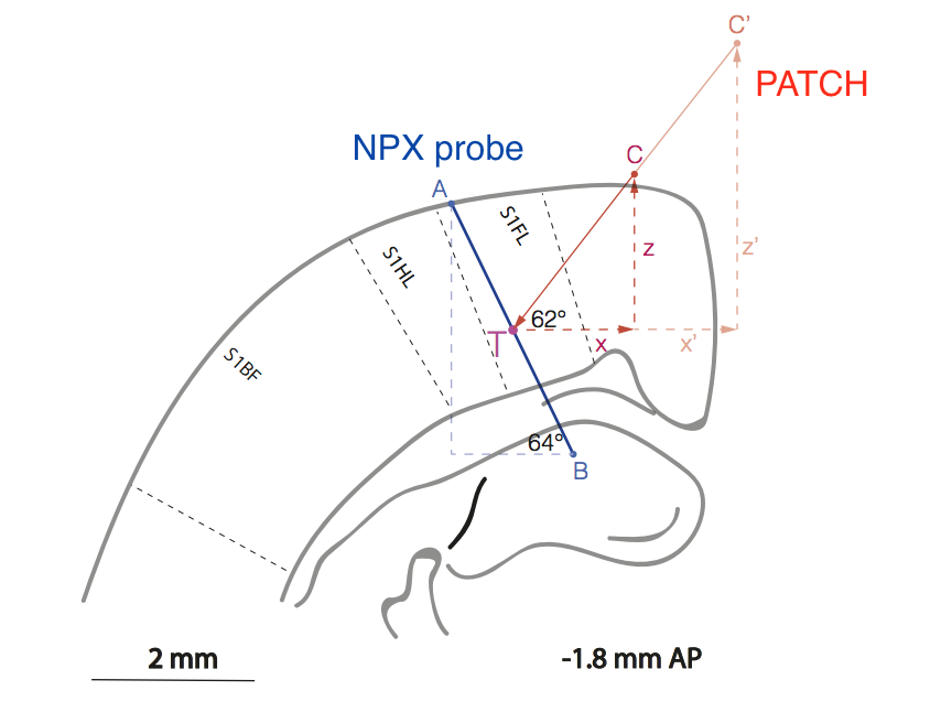
Fig. Schematic representation of the relative position of the sample (line AB) and the patch pipette (line C'CT) in the area of the rat cortex responsible for processing sensory information from the front paw (S1FL = sensory cortex 1 forelimb.
Needless to say that the work is extremely difficult methodologically because experimenters had to develop a method for the mutual arrangement of two electrodes in the cerebral cortex without visual inspection with an accuracy of ~ 10 μm.
Why is it so important to increase the density of registration sites? For analogy, let us take the fact known among EEG researchers that, from a certain threshold, an increase in the number of electrodes in a cap does not lead to a noticeable increase in the information received, that is, the signal from the electrode is slightly different from the linear interpolation of signals from neighboring electrodes. Someone says that this threshold is reached already at 30, someone - at 50, someone - at 100 electrodes. Who works in detail with the EEG can correct. But in the case of cellular activity, the threshold of density of registration sites on one sample is not yet known, therefore the race of high-density samples continues. For this, the Kampff Lab team continues to work with the sample with a 5x5 micron 2 site , and for this we have posted preliminary data. Specialists working with dense electrodes share experience that, unexpectedly, the specific number of individual cells that can be isolated from samples of the same area is higher where the density of registration sites is higher. This effect is well illustrated in another study by the same coauthors, where only part of the sites with dense samples were artificially selected and the quality of the obtained clusters after tSNE conversion on PCA values from waveforms of spikes was visually assessed. This is not a canon for clustering, but it is good for illustrating dependencies. As a test, the work was performed by the Neuroseeker on 128 channels with a total size of 700x70 µm 2 with a site of 20x20 µm 2 .

Fig. Diagrams tSNE over PCA on wet waveforms with artificial decrease of site density on the sample. Work sites are shown schematically on top of each chart. It is clearly shown how exactly the number of segregated clusters grows with an increase in the density of sites, A is the best, F is the worst.
In the data, Marques-Smith et al. There are simultaneous recordings of patch clamp and samples. Using data from a patch clamp, scientists found moments of action potentials and used these moments to segment and average the waveforms already in the sample. As a result, they were able to build very high-quality distributions of the action potential in time and space over the entire sample area.

Fig. On the left are traces of cell activity simultaneously in the patch clamp (black) and on the nearest of the Neuropixels channels (blue). In the middle - 500 individual samples and their averaging. On the right is the distribution of the action potential in space over the sample area and in time.
Further on, the question of the variation of extracellular waveform from spike to spike is raised - yes, it is tangible and should be taken into account. Then they show that it is fundamentally possible to track the spread of the action potential across the cell membrane with the help of its dense electrodes, but this has already been shown earlier in the works of other groups. In conclusion, they offer potential collaborators some fundamental questions from neurophysiology that can be tried to be answered using their datasets, and also suggest using datasets to validate the pipelines for clustering cellular activity. The latter sounds like a bold challenge, because now there is a lot of clustering algorithms, and the competition among the methods is very large. Not every method, firstly, works with such a large number of channels, and, secondly,
First, a new version of Neuroseeker for 1300 channels is also on the way, also on CMOS technologies, preliminary data are already available .
Secondly, we are waiting for another datasset, already from the Allen Institute for Brain Science, which was announced at the FENS conference in 2018. It will simultaneously use 4 (!) Neuropixels samples to study the visual cortex of mice with various visual stimuli. They promised to publish at the end of 2018 here , next to the data on the biphoton (also very powerful dataset), but so far nothing.
Third, the task of clustering cells from recording extracellular potential seems to me aesthetically beautiful. It converges methods of microelectronics, neurophysiology and machine learning. In addition, it has great fundamental and applied value. I suppose that the audience of Habr will be interested to learn about the technical kitchen of electrophysiology, namely about the clustering algorithms, because in this area has developed its own zoo. I, in turn, have accumulated several questions to these algorithms, but this one cannot be missed. Therefore, in the next part, we will proceed to the analysis of some algorithms, starting with the canonical Klustakwik, continuing with the standard Kilosort or Spyking Circus methods, and then YASS, which declares itself very stronglythat works faster and better than everyone else, because DL and because it can. A github topic with a list of some clusterers here . Anticipating some issues, I do not see the point in developing my own algorithm, because the competition is already very large, and a lot of ideas have already been implemented and tested by others. But if there are brave souls, I will gladly contribute.
Suggestions and suggestions are accepted. Thanks for attention!
KDPV: the result of modeling the extracellular potential near one neuron in the generation of action potential ( source ). The color indicates the amplitude of the potential. This illustration will be important for further understanding.
Electrophysiological research methodsbrain based on the recording of the electrical potential of the brain. They can be divided into non-invasive - mainly electroencephalography (EEG), and invasive, for example, electrocorticography (ECOG, ECoG), patch clamp (patch-clamp) or registration of local field potential (BOB = local field potentials, LFP) . For the latter, a small electrode with a size of 10-100 μm is injected directly into the brain and its potential is recorded. In order to investigate the mammalian brain activity at the cellular level, i.e., to measure the activity of individual cells, the available non-invasive methods cannot be applied, because the potential from one cell decays in space very quickly, literally over 100 microns (see KDPV). Therefore, in any animal model, as in man,
But with invasive methods is not so simple. To record the activity of a neuron, it is necessary to bring the electrode very close to the neuron, ideally place it inside the cell, as is done in the patch clamp, or with the help of Sharp electrodesthat in practice is difficult, very difficult. On the other hand, any extracellular electrode with a size of ~ 10 μm will register action potentials from 5-10 cells around due to high density of neurons and high ionic conductivity of the extracellular solution. Therefore, the task of registering individual cells is technically resolved by increasing the density of electrodes in the vicinity of the cell. In this regard, modern electrophysiology is moving in the direction of increasing the density of the electrodes, increasing their number and reducing the size. Even among the requirements, there is a need to amplify the signal closer to the registration site, in order to reduce noise, and place a multiplexer to reduce its size. So, in 2016 it was announced in the preprint, and in 2017 it was published in Nature, and in 2018 it was already on the market, a new high-density sample Neuropixels, made by CMOS technology, on 960 electrodes, of which any 384 are available for simultaneous recording. The size of one registration site is 12 microns. The sample thickness is 24 microns. Moreover, with high-density electrodes, as well as with active amplification, people began to work a long time ago, but Neuropixels was the first to reach production and sales, therefore, in the near future, this test will be encountered more and more often in articles.
Fig. Neuropixels scheme. 960 sites are located on a monolithic silicon substrate, as well as a full-fledged multiplexer and an AD interface with 384 channels.
Data structure
In addition to the classic activity rhythms (alpha, beta, gamma, etc.) responsible for group synchronization, the data obtained using similar samples also contain the action potentials of individual cells (PD = action potentials, AP, spikes, spikes) , which on the record look like short peaks with a duration of ~ 1 ms.
Fig. Signals Neuropixels. Two parts of the signal are distinguished: local field potential (LFP, up to ~ 300 Hz) and cellular activity (AP, from 300 Hz).
Moreover, if the low-frequency local field potential is usually analyzed within the framework of oscillations and spectral or wavelet analysis is used as in the EEG, then the cellular activity contains the action potentials of individual cells, it consists of discrete events against the background of noise. The task of isolating the activity of individual cells is formally reduced to the cocktail party problem, when it is necessary to select a separate speaker from a multitude of speakers. Big data appears when we evaluate the data stream from one such sample. For the analysis of spikes, sampling is carried out at 30–40 kHz with digitization from 16 bits per point (uint16), thus, recording already 100 electrodes for 1 second will weigh from 8 MB. At the same time, experiments usually last hours, which amounts to hundreds of gigabytes from just one working day, and for a full-fledged study you need, say, from 10 such records. Therefore, the potential of this sample also strongly depends on the machine learning algorithms that are used for data analysis.
Machine learning and cellular activity
A typical pipeline for analyzing cellular activity consists of preprocessing, segmentation of spikes and clustering. This part of the research is usually referred to as cluster analysis or spike sorting. Low frequency filtering (> 300 Hz) is usually used as preprocessing, because it is considered that there are no other physiological rhythms above 300 Hz, and only information about individual cellular activity remains. Also during preprocessing in dense samples, it is possible to reduce correlated noise, for example, 50 Hz interference. Segmentation is often taken as a simple threshold, for example, everything above 5 standard deviations of noise can be considered an event. It happens that two-threshold segmentation is used, with a soft and hard threshold, to highlight related events in space and time, as in the watershed algorithm (watershed segmentation ), only in clustering spikes does the distribution of markers take into account the sample topology. After segmentation, a window with a duration of 1-2 ms is taken near the center of each event, and the signal in this window, collected from all channels, becomes a sample for further clustering. This sample is called a spike waveform. Different cells and their different distances from the registration site lead to the fact that their waveforms will differ (see CDRV). As the waveform clustering algorithm itself, EM, template match (template match), deep learning and many variations are used ( topic on github). The only requirement is learning without a teacher. But there is one problem. No one knows for sure what parameters you need to take for your pipeline to make the analysis most effective. Usually, after clustering, the analyst manually passes through the results and makes changes at discretion. Thus, the analysis results can include both algorithm errors and human errors. And they may not be, therefore the question of objective validation remains open.
Validating pipeline can be in several ways. First, changing the external conditions for the object of study. For example, during the experiment, if you study the visual cortex, then you can change the texture, color, brightness of the image. If there is a cell in the analysis that changes its activity depending on the stimulus, then you are lucky. Secondly, you can pharmacologically enhance or reduce the activity of a particular cell type, for example, using blockers of certain channels. Then the activity of your cell will increase / decrease, and you will see the difference in clustering. However, this modulation of activity will also lead to changes in waveforms, because the profile of the action potential over time is completely determined by the kinetics of ion channels. Thirdly, you can optogenetically or using a patch pipette, as in this dataset, measure or induce the activity of certain cells. Due to the large signal-to-noise ratio and the stability of the patch electrode, you will be completely confident in the activity of a single cell. Conceptually, the publication was devoted to assembling a validating dataset using a patch clamp.
Fig. Schematic representation of the relative position of the sample (line AB) and the patch pipette (line C'CT) in the area of the rat cortex responsible for processing sensory information from the front paw (S1FL = sensory cortex 1 forelimb.
Needless to say that the work is extremely difficult methodologically because experimenters had to develop a method for the mutual arrangement of two electrodes in the cerebral cortex without visual inspection with an accuracy of ~ 10 μm.
The effect of electrode density on spike clustering
Why is it so important to increase the density of registration sites? For analogy, let us take the fact known among EEG researchers that, from a certain threshold, an increase in the number of electrodes in a cap does not lead to a noticeable increase in the information received, that is, the signal from the electrode is slightly different from the linear interpolation of signals from neighboring electrodes. Someone says that this threshold is reached already at 30, someone - at 50, someone - at 100 electrodes. Who works in detail with the EEG can correct. But in the case of cellular activity, the threshold of density of registration sites on one sample is not yet known, therefore the race of high-density samples continues. For this, the Kampff Lab team continues to work with the sample with a 5x5 micron 2 site , and for this we have posted preliminary data. Specialists working with dense electrodes share experience that, unexpectedly, the specific number of individual cells that can be isolated from samples of the same area is higher where the density of registration sites is higher. This effect is well illustrated in another study by the same coauthors, where only part of the sites with dense samples were artificially selected and the quality of the obtained clusters after tSNE conversion on PCA values from waveforms of spikes was visually assessed. This is not a canon for clustering, but it is good for illustrating dependencies. As a test, the work was performed by the Neuroseeker on 128 channels with a total size of 700x70 µm 2 with a site of 20x20 µm 2 .
Fig. Diagrams tSNE over PCA on wet waveforms with artificial decrease of site density on the sample. Work sites are shown schematically on top of each chart. It is clearly shown how exactly the number of segregated clusters grows with an increase in the density of sites, A is the best, F is the worst.
What is the essence of work
In the data, Marques-Smith et al. There are simultaneous recordings of patch clamp and samples. Using data from a patch clamp, scientists found moments of action potentials and used these moments to segment and average the waveforms already in the sample. As a result, they were able to build very high-quality distributions of the action potential in time and space over the entire sample area.
Fig. On the left are traces of cell activity simultaneously in the patch clamp (black) and on the nearest of the Neuropixels channels (blue). In the middle - 500 individual samples and their averaging. On the right is the distribution of the action potential in space over the sample area and in time.
Further on, the question of the variation of extracellular waveform from spike to spike is raised - yes, it is tangible and should be taken into account. Then they show that it is fundamentally possible to track the spread of the action potential across the cell membrane with the help of its dense electrodes, but this has already been shown earlier in the works of other groups. In conclusion, they offer potential collaborators some fundamental questions from neurophysiology that can be tried to be answered using their datasets, and also suggest using datasets to validate the pipelines for clustering cellular activity. The latter sounds like a bold challenge, because now there is a lot of clustering algorithms, and the competition among the methods is very large. Not every method, firstly, works with such a large number of channels, and, secondly,
What's next
First, a new version of Neuroseeker for 1300 channels is also on the way, also on CMOS technologies, preliminary data are already available .
Secondly, we are waiting for another datasset, already from the Allen Institute for Brain Science, which was announced at the FENS conference in 2018. It will simultaneously use 4 (!) Neuropixels samples to study the visual cortex of mice with various visual stimuli. They promised to publish at the end of 2018 here , next to the data on the biphoton (also very powerful dataset), but so far nothing.
Third, the task of clustering cells from recording extracellular potential seems to me aesthetically beautiful. It converges methods of microelectronics, neurophysiology and machine learning. In addition, it has great fundamental and applied value. I suppose that the audience of Habr will be interested to learn about the technical kitchen of electrophysiology, namely about the clustering algorithms, because in this area has developed its own zoo. I, in turn, have accumulated several questions to these algorithms, but this one cannot be missed. Therefore, in the next part, we will proceed to the analysis of some algorithms, starting with the canonical Klustakwik, continuing with the standard Kilosort or Spyking Circus methods, and then YASS, which declares itself very stronglythat works faster and better than everyone else, because DL and because it can. A github topic with a list of some clusterers here . Anticipating some issues, I do not see the point in developing my own algorithm, because the competition is already very large, and a lot of ideas have already been implemented and tested by others. But if there are brave souls, I will gladly contribute.
Suggestions and suggestions are accepted. Thanks for attention!