Learn OpenGL. Lesson 5.4 - Omnidirectional Shadow Maps
- Transfer
- Tutorial

Omnidirectional shadow maps
In the previous lesson, we figured out how to create dynamic projection shadows. This technique works great, but, alas, it is only suitable for directional light sources, since a shadow map is created in one direction that matches the direction of the source. That is why this technique is also called a directional shadow map, since a depth map (shadow map) is created precisely along the direction of the light source.
This lesson will be devoted to creating dynamic shadows that project in all directions. This approach is great for working with spotlights, because they should cast shadows in all directions at once. Accordingly, this technique is called an omnidirectional shadow map .
The lesson relies heavily on the materials of the previous lesson , so if you have not practiced with regular shadow maps, you should do this before continuing to study this article.
Content
Part 1. Getting Started
Part 2. Basic lighting
Part 3. Download 3D models
Part 4. Advanced OpenGL Features
Part 5. Advanced Lighting
Part 6. PBR
- Opengl
- Window creation
- Hello window
- Hello triangle
- Shaders
- Textures
- Transformations
- Coordinate systems
- Camera
Part 2. Basic lighting
Part 3. Download 3D models
Part 4. Advanced OpenGL Features
- Depth test
- Stencil test
- Color mixing
- Clipping faces
- Frame buffer
- Cubic cards
- Advanced data handling
- Advanced GLSL
- Geometric shader
- Instancing
- Smoothing
Part 5. Advanced Lighting
- Advanced lighting. Blinn-Fong model.
- Gamma correction
- Shadow cards
- Omnidirectional shadow maps
- Normal mapping
- Parallax mapping
- HDR
- Bloom
- Deferred rendering
- SSAO
Part 6. PBR
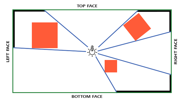
In general, the operation algorithm remains almost identical to that for directional shadows: we create a depth map from the point of view of the light source and for each fragment we compare the values of its depth and the one read from the depth map. The main difference between a directional and omnidirectional approach in the type of depth map used.
The shadow map that we need implies rendering the scene in all directions around the light source and the usual 2D texture is not good here. So maybe use a cubic map ? Since the cubic map can store environmental data with just six faces, you can draw the entire scene on each of these faces and then select the depth from the cubic map.
The created cubic shadow map eventually ends up in the fragment shader, where it is sampled using the direction vector to obtain the fragment depth value (from the point of view of the source). We have already discussed most of the technically complex details in the previous lesson, so there remains one subtlety - the use of a cubic map.
Create a cubic map
To create a cubic map that stores the depth of the light source, we need to render the scene six times: once for each face of the map. One of the (obvious) ways to do this is to simply draw the scene six times using six different view matrices, and in each pass, connect a separate face of the cubic map to the color of the frame buffer object:
for(unsigned int i = 0; i < 6; i++)
{
    GLenum face = GL_TEXTURE_CUBE_MAP_POSITIVE_X + i;
    glFramebufferTexture2D(GL_FRAMEBUFFER, GL_DEPTH_ATTACHMENT, face, depthCubemap, 0);
    BindViewMatrix(lightViewMatrices[i]);
    RenderScene();
}
This approach can be quite expensive in terms of performance, as many draw calls are made to create a single shadow map. In the lesson, we will try to implement a more optimal approach, using a little trick associated with using a geometric shader. This will create a cubic depth map in just one pass.
First, create a cubic map:
unsigned int depthCubemap;
glGenTextures(1, &depthCubemap);
And we set each face as a 2D texture that stores depth values:
const unsigned int SHADOW_WIDTH = 1024, SHADOW_HEIGHT = 1024;
glBindTexture(GL_TEXTURE_CUBE_MAP, depthCubemap);
for (unsigned int i = 0; i < 6; ++i)
        glTexImage2D(GL_TEXTURE_CUBE_MAP_POSITIVE_X + i, 0, GL_DEPTH_COMPONENT,
                     SHADOW_WIDTH, SHADOW_HEIGHT, 0, GL_DEPTH_COMPONENT, GL_FLOAT, NULL);
Also, do not forget to set the appropriate texture parameters:
glTexParameteri(GL_TEXTURE_CUBE_MAP, GL_TEXTURE_MAG_FILTER, GL_NEAREST);
glTexParameteri(GL_TEXTURE_CUBE_MAP, GL_TEXTURE_MIN_FILTER, GL_NEAREST);
glTexParameteri(GL_TEXTURE_CUBE_MAP, GL_TEXTURE_WRAP_S, GL_CLAMP_TO_EDGE);
glTexParameteri(GL_TEXTURE_CUBE_MAP, GL_TEXTURE_WRAP_T, GL_CLAMP_TO_EDGE);
glTexParameteri(GL_TEXTURE_CUBE_MAP, GL_TEXTURE_WRAP_R, GL_CLAMP_TO_EDGE);
In the usual approach, we would connect each face of the cubic map to the frame buffer and render the scene six times, in each pass, replacing the face of the cubic map connected to the depth attachment of the frame buffer. But using the geometric shader, we can bring the scene to all sides at once in one pass, and therefore we connect the cubic map directly to the depth attachment:
glBindFramebuffer(GL_FRAMEBUFFER, depthMapFBO);
glFramebufferTexture(GL_FRAMEBUFFER, GL_DEPTH_ATTACHMENT, depthCubemap, 0);
glDrawBuffer(GL_NONE);
glReadBuffer(GL_NONE);
glBindFramebuffer(GL_FRAMEBUFFER, 0);
And again, I note the calls to glDrawBuffer and glReadBuffer : since only depth values are important to us, we explicitly tell OpenGL that we can not write to the color buffer.
Ultimately, two passes will be applied here: the shadow map is prepared first, the scene is drawn second, and the map is used to create the shading. Using a framebuffer and a cubic map, the code looks something like this:
// 1. рендер в кубическую карту глубин
glViewport(0, 0, SHADOW_WIDTH, SHADOW_HEIGHT);
glBindFramebuffer(GL_FRAMEBUFFER, depthMapFBO);
    glClear(GL_DEPTH_BUFFER_BIT);
    ConfigureShaderAndMatrices();
    RenderScene();
glBindFramebuffer(GL_FRAMEBUFFER, 0);
// 2. обычный рендер сцены с использованием кубической карты глубин для затенения
glViewport(0, 0, SCR_WIDTH, SCR_HEIGHT);
glClear(GL_COLOR_BUFFER_BIT | GL_DEPTH_BUFFER_BIT);
ConfigureShaderAndMatrices();
glBindTexture(GL_TEXTURE_CUBE_MAP, depthCubemap);
RenderScene();
In a first approximation, the process is the same as using directional shadow maps. The only difference is that we render to a cubic depth map, and not to the usual 2D texture.
Before we start directly rendering the scene from directions relative to the source, we need to prepare suitable transformation matrices.
Convert to light coordinate system
Having a prepared frame buffer object and a cubic map, we turn to the question of transforming all scene objects into coordinate spaces corresponding to all six directions from the light source. We compose the transformation matrices in the same way as in the previous lesson , but this time we need a separate matrix for each face.
Each final transformation into the source space contains both a projection matrix and a species matrix. For the projection matrix, we use the perspective projection matrix: the source is a point in space, so the perspective projection is most suitable here. This matrix will be the same for all final transformations:
float aspect = (float)SHADOW_WIDTH/(float)SHADOW_HEIGHT;
float near = 1.0f;
float far = 25.0f;
glm::mat4 shadowProj = glm::perspective(glm::radians(90.0f), aspect, near, far);
I note an important point: the viewing angle parameter during matrix formation is set to 90 °. It is this value of the viewing angle that provides us with a projection that allows us to correctly fill the faces of the cubic map so that they converge without gaps.
Since the projection matrix remains constant, you can reuse the same matrix to create all six matrices of the final transformation. But species matrices are needed unique for each facet. Using glm :: lookAt, we will create six matrices representing six directions in the following order: right, left, top, bottom, near face, far side:
std::vector shadowTransforms;
shadowTransforms.push_back(shadowProj *
                 glm::lookAt(lightPos, lightPos + glm::vec3( 1.0, 0.0, 0.0), glm::vec3(0.0,-1.0, 0.0));
shadowTransforms.push_back(shadowProj *
                 glm::lookAt(lightPos, lightPos + glm::vec3(-1.0, 0.0, 0.0), glm::vec3(0.0,-1.0, 0.0));
shadowTransforms.push_back(shadowProj *
                 glm::lookAt(lightPos, lightPos + glm::vec3( 0.0, 1.0, 0.0), glm::vec3(0.0, 0.0, 1.0));
shadowTransforms.push_back(shadowProj *
                 glm::lookAt(lightPos, lightPos + glm::vec3( 0.0,-1.0, 0.0), glm::vec3(0.0, 0.0,-1.0));
shadowTransforms.push_back(shadowProj *
                 glm::lookAt(lightPos, lightPos + glm::vec3( 0.0, 0.0, 1.0), glm::vec3(0.0,-1.0, 0.0));
shadowTransforms.push_back(shadowProj *
                 glm::lookAt(lightPos, lightPos + glm::vec3( 0.0, 0.0,-1.0), glm::vec3(0.0,-1.0, 0.0));
In the above code, the six created view matrices are multiplied by the projection matrix to specify six unique matrices to transform into the space of the light source. The target parameter in the call to glm :: lookAt represents the direction of the look at each of the faces of the cubic map.
Further, this list of matrices is passed to the shaders when rendering a cubic depth map.
Depth Shaders
To write depth to a cubic map, we use three shaders: vertex, fragment, and additional geometric, which runs between these stages.
It is the geometric shader that will be responsible for converting all the vertices in world space into six separate spaces of the light source. Thus, the vertex shader is trivial and simply gives the coordinates of the vertex in the world space, which will go to the geometric shader:
#version 330 core
layout (location = 0) in vec3 aPos;
uniform mat4 model;
void main()
{
    gl_Position = model * vec4(aPos, 1.0);
}
The geometric shader accepts at the input three vertices of the triangle, as well as uniforms with an array of transformation matrices into the spaces of the light source. Here lies an interesting point: it is the geometric shader that will be involved in the conversion of vertices from world coordinates to source spaces.
The built-in variable gl_Layer is available for the geometric shader, which sets the face number of the cubic map for which the shader will form the primitive. In a normal situation, the shader simply sends all the primitives further to the pipeline without any further action. But we can control the change in the value of this variable to which face of the cubic map we are going to render each of the processed primitives. Of course, this only works if a cubic card is connected to the frame buffer.
#version 330 core
layout (triangles) in;
layout (triangle_strip, max_vertices=18) out;
uniform mat4 shadowMatrices[6];
// переменная FragPos вычисляется в геометрическом шейдере
// и выдается для каждого вызова EmitVertex()
out vec4 FragPos;
void main()
{
    for(int face = 0; face < 6; ++face)
    {
        // встроенная переменная, определяющая в какую
        // грань кубической карты идет рендер
        gl_Layer = face;
        for(int i = 0; i < 3; ++i) // цикл по всем вершинам треугольника
        {
            FragPos = gl_in[i].gl_Position;
            gl_Position = shadowMatrices[face] * FragPos;
            EmitVertex();
        }
        EndPrimitive();
    }
}
The code presented should be pretty straightforward. The shader receives a triangle-type primitive at the input, and produces six triangles (6 * 3 = 18 vertices) as the result. In the main function, we loop through all six faces of the cubic map, setting the current index as the number of the active face of the cubic map with the corresponding entry in the gl_Layer variable . We also transform each input vertex from the world coordinate system into the space of the light source corresponding to the current face of the cubic art. For this, FragPos is multiplied by a suitable transform matrix from the uniform array shadowMatrices . Note that the FragPos value is also passed to the fragment shader to calculate the fragment depth.
In the last lesson, we used an empty fragment shader, and OpenGL itself was busy calculating the depth for the shadow map. This time we will manually form a linear depth value, taking as a basis the distance between the position of the fragment and the light source. Such a calculation of the depth value makes subsequent shading calculations a little more intuitive.
#version 330 core
in vec4 FragPos;
uniform vec3 lightPos;
uniform float far_plane;
void main()
{
    // вычисление расстояния между фрагментом и источником
    float lightDistance = length(FragPos.xyz - lightPos);
    // преобразование к интервалу [0, 1] посредством деления на far_plane
    lightDistance = lightDistance / far_plane;
    // запись результата в результирующую глубину фрагмента
    gl_FragDepth = lightDistance;
}
The FragPos variable from the geometric shader, the source position vector, as well as the distance to the far clipping plane of the pyramid of the projection of the light source gets to the input of the fragment shader . In this code, we simply calculate the distance between the fragment and the source, bring it to the range of values [0., 1.] and write it as a result of the shader.
A scene renderer with these shaders and a cubic map connected to the frame buffer object should generate a fully prepared shadow map for use in the next render pass.
Omnidirectional shadow maps
Once everything is prepared for us, then we can proceed to the direct rendering of omnidirectional shadows. The procedure is similar to that presented in the previous lesson for directional shadows, but this time we use a cubic texture instead of a two-dimensional one as a depth map, and also transfer uniforms with the value of the far plane of the projection pyramid for the light source to the shaders.
glViewport(0, 0, SCR_WIDTH, SCR_HEIGHT);
glClear(GL_COLOR_BUFFER_BIT | GL_DEPTH_BUFFER_BIT);
shader.use();
// ... передача данных юниформов в шейдер (включая параметр матрицы проекции источника света far_plane)
glActiveTexture(GL_TEXTURE0);
glBindTexture(GL_TEXTURE_CUBE_MAP, depthCubemap);
// ... привязка текстур
RenderScene();
In the example, the renderScene function displays several cubes located in a large cubic room that will cast shadows from the light source located in the center of the scene.
The vertex and fragment shaders are almost identical to those discussed in the lesson on directional shadows. So, in the fragment shader, the input parameter for the position of the fragment in the space of the light source is no longer required, since the selection from the shadow map is now done using the direction vector.
The vertex shader, respectively, now does not have to convert the position vector into the space of the light source, so that we can throw out the FragPosLightSpace variable :
#version 330 core
layout (location = 0) in vec3 aPos;
layout (location = 1) in vec3 aNormal;
layout (location = 2) in vec2 aTexCoords;
out vec2 TexCoords;
out VS_OUT {
    vec3 FragPos;
    vec3 Normal;
    vec2 TexCoords;
} vs_out;
uniform mat4 projection;
uniform mat4 view;
uniform mat4 model;
void main()
{
    vs_out.FragPos = vec3(model * vec4(aPos, 1.0));
    vs_out.Normal = transpose(inverse(mat3(model))) * aNormal;
    vs_out.TexCoords = aTexCoords;
    gl_Position = projection * view * model * vec4(aPos, 1.0);
}
The code of the Blinn-Fong lighting model in the fragment shader remains untouched, it also leaves a multiplication by the shading coefficient at the end:
#version 330 core
out vec4 FragColor;
in VS_OUT {
    vec3 FragPos;
    vec3 Normal;
    vec2 TexCoords;
} fs_in;
uniform sampler2D diffuseTexture;
uniform samplerCube depthMap;
uniform vec3 lightPos;
uniform vec3 viewPos;
uniform float far_plane;
float ShadowCalculation(vec3 fragPos)
{
    [...]
}
void main()
{
    vec3 color = texture(diffuseTexture, fs_in.TexCoords).rgb;
    vec3 normal = normalize(fs_in.Normal);
    vec3 lightColor = vec3(0.3);
    // фоновое освещение
    vec3 ambient = 0.3 * color;
    // диффузный компонент
    vec3 lightDir = normalize(lightPos - fs_in.FragPos);
    float diff = max(dot(lightDir, normal), 0.0);
    vec3 diffuse = diff * lightColor;
    // зеркальная компонента
    vec3 viewDir = normalize(viewPos - fs_in.FragPos);
    vec3 reflectDir = reflect(-lightDir, normal);
    float spec = 0.0;
    vec3 halfwayDir = normalize(lightDir + viewDir);
    spec = pow(max(dot(normal, halfwayDir), 0.0), 64.0);
    vec3 specular = spec * lightColor;
    // расчет затенения
    float shadow = ShadowCalculation(fs_in.FragPos);
    vec3 lighting = (ambient + (1.0 - shadow) * (diffuse + specular)) * color;
    FragColor = vec4(lighting, 1.0);
}
I also note a few subtle differences: the lighting model code is really unchanged, but now a samplerCubemap type sampler is used , and the ShadowCalculation function takes the coordinates of the fragment in world coordinates, instead of the space of the light source. We also use the far_plane light source projection pyramid parameter in further calculations. At the end of the shader, we calculate the shading factor, which is 1 when the fragment is in the shadow; or 0 when the fragment is outside the shadow. This coefficient is used to influence the prepared values of the diffuse and mirror components of lighting.
The biggest changes concern the body of the ShadowCalculation function., where depth values are now sampled from a cubic map rather than a 2D texture. Let's analyze the code of this function in order.
The first step is to get the direct depth value from the cubic map. As you remember, in preparing the cubic map, we wrote down the depth in it, which is represented as the distance between the fragment and the light source. The same approach is used here:
float ShadowCalculation(vec3 fragPos)
{
    vec3 fragToLight = fragPos - lightPos;
    float closestDepth = texture(depthMap, fragToLight).r;
}
The difference vector between the position of the fragment and the light source is calculated, which is used as the direction vector for sampling from the cubic map. As we recall, the sample vector from a cubic map does not have to have a unit length, then there is no need to normalize it. The resulting closestDepth value is the normalized depth value of the nearest visible fragment relative to the light source.
Since the value of closestDepth is in the interval [0., 1.], you must first perform the inverse conversion to the interval [0., far_plane ]:
closestDepth *= far_plane; Next, we get the depth value for the current fragment relative to the light source. For the chosen approach, it is extremely simple: you just need to calculate the length of the already prepared fragToLight vector :
float currentDepth = length(fragToLight); Thus, we obtain a depth value lying in the same (and, possibly, in a larger) interval as closestDepth .
Now we can begin to compare both depths in order to find out whether the current fragment is in the shadow or not. We also immediately include the offset value in the comparison so as not to run into the “shadow ripple” problem explained in the previous lesson :
float bias = 0.05;
float shadow = currentDepth -  bias > closestDepth ? 1.0 : 0.0;
Full ShadowCalculation Code :
float ShadowCalculation(vec3 fragPos)
{
// расчет вектора между положением фрагмента и положением источника света
vec3 fragToLight = fragPos - lightPos;
// полученный вектор направления от источника к фрагменту
// используется для выборки из кубической карты глубин
float closestDepth = texture(depthMap, fragToLight).r;
// получено линейное значение глубины в диапазоне [0,1]
// проведем обратную трансформацию в исходный диапазон
closestDepth *= far_plane;
// получим линейное значение глубины для текущего фрагмента
// как расстояние от фрагмента до источника света
float currentDepth = length(fragToLight);
// тест затенения
float bias = 0.05;
float shadow = currentDepth - bias > closestDepth ? 1.0 : 0.0;
return shadow;
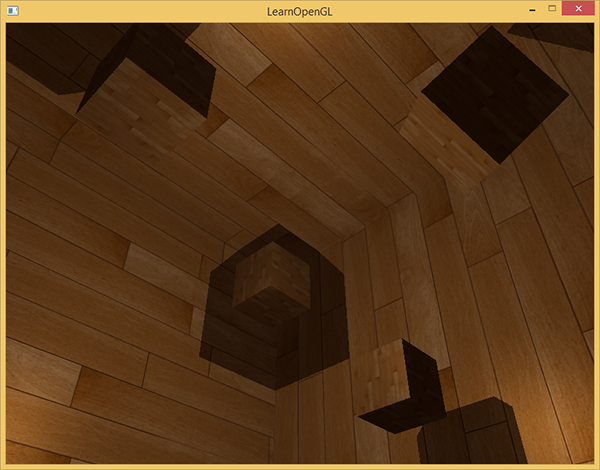
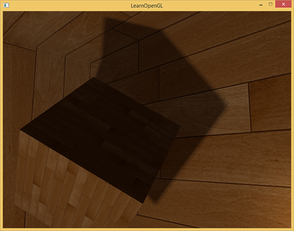
} With the given shaders, the application already displays quite tolerable shadows and this time they are cast in all directions from the source. For a scene with a source in the center, the picture appears as follows:
The full source code is here .
Visualization of a Cubic Map of the Depths
If you are somewhat similar to me, then, I think, the first time you will not be able to do everything right, and therefore some means of debugging the application would be quite useful. As the most obvious option, it would be nice to be able to verify the correctness of the preparation of the depth map. Since we now use a cubic map rather than a two-dimensional texture, the issue of visualization requires a slightly more intricate approach.
A simple way out would be to take the normalized value closestDepth from the body of the ShadowCalculation function and output it as the result of the fragment shader:
FragColor = vec4(vec3(closestDepth / far_plane), 1.0); The result is a scene in grayscale, where the color intensity corresponds to a linear depth value in this scene:
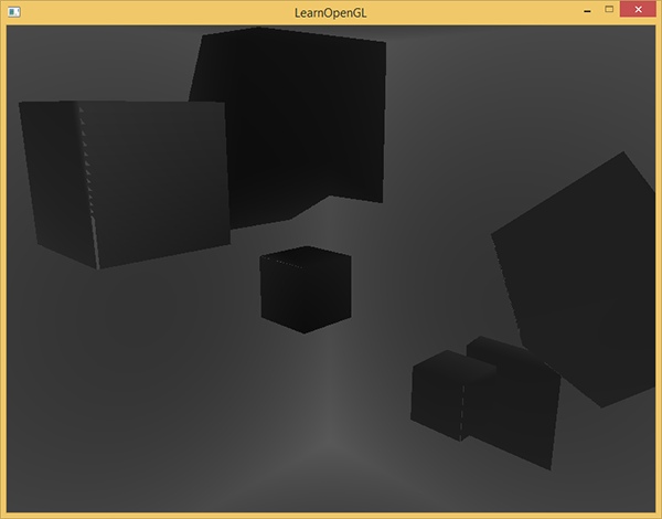
Shading areas on the walls of the room are also visible. If the result of the visualization is similar to the one given, then you can be sure that the shadow maps are prepared correctly. Otherwise, an error crept in somewhere: for example, the value closestDepth was taken from the interval [0., far_plane ].
Percentage-closer filtering
Since omnidirectional shadows are built on the same principles as directional shadows, they inherited all the artifacts associated with the accuracy and finiteness of texture resolution. If you approach the borders of the shaded areas, you will see jagged edges, i.e. aliasing artifacts. Filtering method Percentage-closer filtering ( PCF ) allows to smooth traces aliasing by filtering a plurality of depth samples around the current fragment and the averaging depth comparison result.
Take the PCF code from the previous lesson and add the third dimension (a sample from a cubic map does require a direction vector):
float shadow  = 0.0;
float bias    = 0.05;
float samples = 4.0;
float offset  = 0.1;
for(float x = -offset; x < offset; x += offset / (samples * 0.5))
{
    for(float y = -offset; y < offset; y += offset / (samples * 0.5))
    {
        for(float z = -offset; z < offset; z += offset / (samples * 0.5))
        {
            float closestDepth = texture(depthMap, fragToLight + vec3(x, y, z)).r;
            closestDepth *= far_plane;   // обратное преобразование из диапазона [0;1]
            if(currentDepth - bias > closestDepth)
                shadow += 1.0;
        }
    }
}
shadow /= (samples * samples * samples);
There are few differences. We calculate the displacements for the texture coordinates dynamically, based on the number of samples that we want to make on each axis and average the result by dividing by the number of samples cubed.
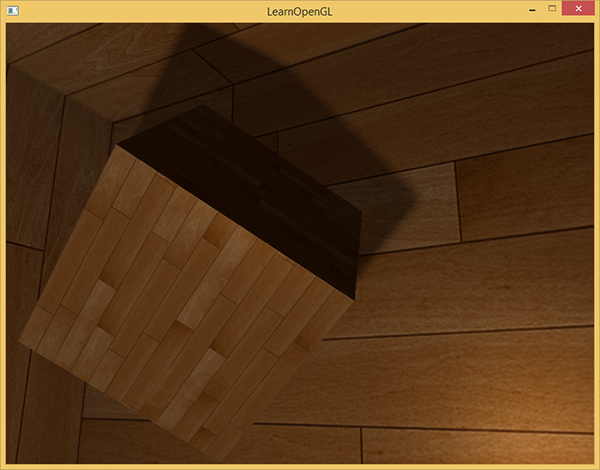
Now the shadows look much more authentic and their edges are quite smooth.
However, setting the number of samples samples = 4 , we will in fact spend as many as 64 samples for each fragment, which is a lot.
And in most cases, these samples will be redundant, because they will be very close to the original vector of the sample. Perhaps it would be more useful to make samples in directions perpendicular to the original vector of the sample. Alas, a simple method for finding out which of the additional directions generated would be redundant does not exist. You can use one trick and ask yourself an array of bias directions, which are all almost completely separable vectors, i.e. each of them will point in completely different directions. This will reduce the number of bias directions that are too close to each other. Below is just a similar array with twenty specially selected directions of displacement:
vec3 sampleOffsetDirections[20] = vec3[]
(
   vec3( 1,  1,  1), vec3( 1, -1,  1), vec3(-1, -1,  1), vec3(-1,  1,  1),
   vec3( 1,  1, -1), vec3( 1, -1, -1), vec3(-1, -1, -1), vec3(-1,  1, -1),
   vec3( 1,  1,  0), vec3( 1, -1,  0), vec3(-1, -1,  0), vec3(-1,  1,  0),
   vec3( 1,  0,  1), vec3(-1,  0,  1), vec3( 1,  0, -1), vec3(-1,  0, -1),
   vec3( 0,  1,  1), vec3( 0, -1,  1), vec3( 0, -1, -1), vec3( 0,  1, -1)
);
Further, we can modify the PCF algorithm to use fixed-size arrays like sampleOffsetDirections in the process of fetching from a cubic map. The main advantage of this approach is the creation of a result that is visually similar to the first approach, but requiring a significantly smaller number of additional samples.
float shadow = 0.0;
float bias   = 0.15;
int samples  = 20;
float viewDistance = length(viewPos - fragPos);
float diskRadius = 0.05;
for(int i = 0; i < samples; ++i)
{
    float closestDepth = texture(depthMap, fragToLight + sampleOffsetDirections[i] * diskRadius).r;
    closestDepth *= far_plane;   // обратное преобразование из диапазона [0;1]
    if(currentDepth - bias > closestDepth)
        shadow += 1.0;
}
shadow /= float(samples);
In the above code, the displacement vector is multiplied by the diskRadius value representing the radius of the disk built around the original fragToLight sample vector and within which additional samples are made.
You can go even further and do the following trick: try changing the diskRadius value in accordance with the distance of the observer from the fragment. So we can increase the radius of displacement and make the shadows softer for distant fragments, sharper for fragments close to the observer:
float diskRadius = (1.0 + (viewDistance / far_plane)) / 25.0; The result of such a PCF algorithm produces soft shadows no worse, if not better, than the original approach:
Of course, the bias value that is added for each fragment is extremely dependent on the context and content of the scene, and therefore will always require additional experimental settings. Experiment with the parameters of the proposed algorithm to see their effect on the final picture.
The source code for the example can be found here .
I also note that using a geometric shader to create a cubic depth map will not necessarily be faster than a six-time rendering of a scene for each of its faces. Using this approach has its own negative effects on performance. It is possible that the negative contribution to performance will generally outweigh the whole benefit of using a geometric shader and a single draw call. And, of course, it depends on what environment you work in, which video card and which drivers are available to you, and many other things. Therefore, if performance is really important to you, then it is always worthwhile to profile all the alternatives under consideration and choose the one that turned out to be the most effective for the scene in the application.
Additional materials:
- Shadow Mapping for point light sources in OpenGL : a tutorial on omnidirectional shadow maps from sunandblackcat .
- Multipass Shadow Mapping With Point Lights : Similar, but from the author of ogldev .
- Omni-directional Shadows : an entertaining presentation on omnidirectional shadow maps by Peter Houska .
PS : We have a telegram conf for coordination of transfers. If you have a serious desire to help with the translation, then you are welcome!