Program for digitizing graphs, drawings, drawings: algorithms of the project "Tutor: mathematics"
- Tutorial
Content
Opening remarks
Principle of work
Description of the program
Final code of the program
Advantages of working with digitized functions using examples
Epilogue
introduction
In various fields related to science and education, engineering, there is a problem associated with obtaining data from graphs created at a time when digital media did not yet exist, or the real data for which the graphs were created were lost, or, finally, the graph is the final form of operation of some devices that do not give out a set of coordinates of points in an explicit form.
In order to obtain data, you need to “ digitize ” such a graph (or graphic object), in other words, you need to get a set of abscissas and ordinates of the graph points - then you can perform various manipulations on them: build a new (high-quality) graph, perform calculations, translating it into a new format (for example, building a spline), etc.
In the project "Tutor: mathematics "(read the article on Habrahabr - " Tutor: mathematics "to prepare for the exam and VPR - from idea to release. A story about a unique educational project ) we met with this problem in two main ways:
- “Digitizing” the graphic in order to make it fit our style or just make it look decent;
- obtaining a set of base points for constructing geometric drawings, histograms, etc. based on the author’s freehand drawing (or using simple graphical systems).
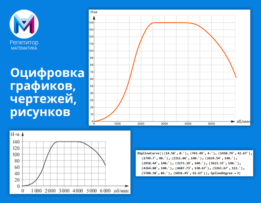
This post provides the code for the graphicsDigitizing function created for this , and also briefly describes how it works. You can also see how it works live .
Principle of operation
The program is quite simple. It is necessary to place a digital illustration (scan, photo, screenshot, other picture) on a certain field on the “first” layer. Next, its manual processing is performed:
- selection of the workspace (rectangle) with the definition of the “real” coordinates of its left lower and upper right vertices - in other words, the definition area and the values of the function (graph, set of points) that we will get as a result;
- setting reference points on which a B-spline of a given degree will be built;
- preview of the result;
- output of the result in a calculated form for further work.
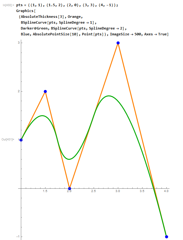
We chose B-splines for several reasons:
- they give flexible curves (if the degree of the B-spline is higher than the 1st),
- give compact analytical representations of the curves ( Bezier curves are a degenerate case of B-splines in which each point, if we simply say, affects the entire form of the curve);
- easy to use (implemented in many packages and not so complicated if you need to program them from scratch yourself).
The figure below shows a set of points (reference points), a set of B-splines of the 1st, 2nd and 3rd degrees, as well as a Bezier curve (in the case shown, this is essentially a 7th degree B-spline).

To create a program for digitizing graphs - as for many other tasks - we use the Wolfram Language .
Program description
Of course, we will not describe how the entire code of the program presented below works step by step , it would be a very long time and, as it seems to us, those who are interested in the issue under discussion or, moreover, those who are urgently facing it, will be able to figure it out themselves in all the “cogs” of the code, fortunately, it is short.
We will pay attention to its main elements.
Let's start with the set of functions that will be required for implementation. You can look at what each of them does in the documentation:
CompoundExpression , ClearAll , SetDelayed , Optional , Pattern , Blank , Image , ImageResize , List, Rule , ColorSpace , With , Set , ImageDimensions , CreateDialog , ExpressionCell , DynamicModule , Grid , DefaultButton , DialogReturn , If , Less , Length , None , Drop , Transpose , Part , Span , ReplaceAll , Rescale , All , Min , Max ,RuleDelayed , Real , Round , CopyToClipboard , BSplineCurve , SplineDegree , TabView , Row , Slider , Dynamic , Times , Pi , Power , ImageSize , Small , Slider2D , SetterBar , InputField , FieldSize , Alignment , Left , Spacings , Automatic , LocatorPane ,Framed , Graphics , Inset , Cos , Sin , EdgeForm , Directive , AbsoluteThickness , RGBColor , Opacity , Yellow , Rectangle , Dashed , Blue , PlotRange , Plus , LocatorAutoCreate , True , Center , Top , Axes , AspectRatio , Initialization , Null ,Condition , String , FileExistsQ , Import , BlankNullSequence , Echo , Inactive , Nothing
One of the main functions in this program is the DynamicModule function for creating interactive spaces and objects. With its help, there is a "revival" of the entire structure.
Function Grid needed for the organization of space - it allows you to build different shapes and tables placed in their cells content: texts, sliders, illustrations, interactive objects, and so on..
Functions LocatorPane , Slider , Slider2D, InputField are used to make interactive elements - a field with a choice of points, sliders (one- and two-dimensional, respectively), a text input field (for the function definition area).
For "drawing" graphic primitives, use the Graphics function (and if necessary in 3D, use Graphics3D ).
And, of course, the BSplineCurve function is the most important here , which allows you to represent a set of points in the form of a finished B-spline curve.
In the video below, you can see how the program works live:
The final code of the program
The final function is actually not as great as it might seem. Although this, of course, is a direct consequence of the great features of Wolfram Language:
View code
ClearAll[graphicsDigitizing];
graphicsDigitizing[image_Image: ImageResize[Image[{{{1,1,1}}},ColorSpace->"RGB"],{600,600}]]:=With[
{im=ImageResize[image,600]},
With[
{imdim=ImageDimensions[im]},
CreateDialog[{
ExpressionCell[
DynamicModule[
{degree,xmin=0,xmax=1,ymin=0,ymax=1,currentFunction,u,unew,udiap,\[Alpha],\[Beta]1,\[Beta]2},
Grid[
{
{
DefaultButton[
"Скопировать сплайн в буфер обмена",
DialogReturn[
With[
{var1=If[
Length[u]<4,
None,
unew=Drop[u,2];
udiap=Transpose[u[[1;;2]]];
Transpose[
{
Rescale[unew[[All,1]],{Min[udiap[[1]]],Max[udiap[[1]]]},{xmin,xmax}],
Rescale[unew[[All,2]],{Min[udiap[[2]]],Max[udiap[[2]]]},{ymin,ymax}]}
]/.x_Real:>Round[x,0.01]],var2=degree},
CopyToClipboard[BSplineCurve[var1,SplineDegree->var2]]]
]]
},
{
TabView[
{"Оригинал"->Grid[
{
{
Grid[
{
{
Row[{"Угол поворота:",Slider[Dynamic@\[Alpha],{-Pi/6,Pi/6},ImageSize->Small]}," "]
},
{
Row[{"Отступы:",Slider2D[Dynamic[\[Beta]1],{0.2 Max[imdim] {-1,-1},0.2 Max[imdim] {1,1}}],Slider2D[Dynamic[\[Beta]2],{0.2 Max[imdim] {-1,-1},0.2 Max[imdim] {1,1}}]}," "]
},
{
Row[{"Степень сплайна:",SetterBar[Dynamic@degree,{0,1,2,3,4}]}," "]
},
{
Grid[{{"\!\(\*SubscriptBox[\(x\), \(min\)]\) =",
InputField[Dynamic[xmin],FieldSize->{3,1}],"\!\(\*SubscriptBox[\(x\), \(max\)]\) =",
InputField[Dynamic[xmax],FieldSize->{3,1}]},{"\!\(\*SubscriptBox[\(y\), \(min\)]\) =",
InputField[Dynamic[ymin],FieldSize->{3,1}],"\!\(\*SubscriptBox[\(y\), \(max\)]\) =",
InputField[Dynamic[ymax],FieldSize->{3,1}]}}]
}},
Alignment->Left,
Spacings->{Automatic,1}],
LocatorPane[
Dynamic@u,
Framed@Dynamic@Graphics[{Inset[im,{0,0},{0,0},imdim,{Cos[\[Alpha]],Sin[\[Alpha]]}],
{EdgeForm[Directive[AbsoluteThickness[3],RGBColor[{214,0,0}/255]]],
Opacity[0.2,Yellow],
Rectangle[u[[1]],u[[2]]]},
{Dashed,Blue,AbsoluteThickness[4],
If[Length[u]<4,BSplineCurve[u[[1;;2]],SplineDegree->2],BSplineCurve[Drop[u,2],SplineDegree->degree]]
}},
PlotRange->Transpose[{\[Beta]1,imdim+\[Beta]2}],ImageSize->600],LocatorAutoCreate->True]
}
},Alignment->{Center,Top}
],
"Результат"->Dynamic@Graphics[
{Blue,AbsoluteThickness[2],
If[Length[u]<4,
BSplineCurve[u[[1;;2]],SplineDegree->2],
BSplineCurve[unew=Drop[u,2];
udiap=Transpose[u[[1;;2]]];
Transpose[
{Rescale[unew[[All,1]],{Min[udiap[[1]]],Max[udiap[[1]]]},{xmin,xmax}],
Rescale[unew[[All,2]],{Min[udiap[[2]]],Max[udiap[[2]]]},{ymin,ymax}]}],
SplineDegree->degree]]},
PlotRange->{{xmin,xmax},{ymin,ymax}},
ImageSize->600,
Axes->True,
AspectRatio->imdim[[2]]/imdim[[1]]]
},Alignment->Center]
}
}
],
Initialization:>(u={{0,0},imdim};\[Alpha]=0;
degree=3;\[Beta]1=0.1 Max[imdim] {-1,-1};\[Beta]2=0.1 Max[imdim] {1,1})]
]}];]];
graphicsDigitizing[image_String/;FileExistsQ[image]]:=graphicsDigitizing[Import[image]];
graphicsDigitizing[x___]:=(Echo[Inactive[graphicsDigitizing][x],"Не подходящие параметры: "];
Nothing)
The advantages of working with digital functions on examples
Naturally, any work is extremely difficult with the graphics before digitization, however, after you digitize the schedule, say, using our program, you can already do a lot. We show some examples.
For example, let’s give a graph:
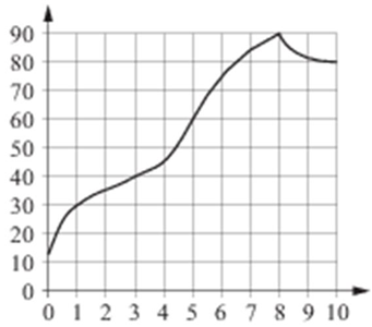
Let's digitize it (see video above ) and make calculations.
To begin with, we only replace the head part of the expression obtained during the work of the program from BSplineCurve to BSplineFunction , which builds an analytical expression with which we can already perform calculations:

The only drawback is that such a function is normalized to 1, i.e., the function f (t) when t changes from 0 to 1, it runs through all its values, which are the points of the B-spline:

However, this is easy to fight. It is enough to build an interpolation polynomial:

After that, you can already do anything.
Build a graph, say, from 1 to 9:

Integrate a function over the entire task area:

Build a graph of the derivative:

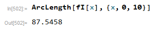
Find the length of the curve:
Or, the analytical representation of the curve (in parametric form):

Code with illustration
pts=Rationalize[{{0.01`,10.92`},{0.19`,16.36`},{0.34`,20.76`},{0.55`,25.17`},{0.96`,29.57`},{1.9100000000000001`,34.49`},{2.74`,38.63`},{3.38`,42.09`},{3.97`,44.03`},{4.47`,49.77`},{4.88`,56.5`},{5.29`,63.24`},{5.65`,69.19`},{6.0600000000000005`,74.63`},{6.53`,78.52`},{7.0200000000000005`,83.96000000000001`},{7.46`,86.55`},{8.02`,89.4`},{8.26`,86.55`},{8.67`,82.4`},{9.21`,80.85000000000001`},{9.57`,79.81`},{9.93`,79.81`}},1/100];
ptsL=Length[pts];
splineDegree=3;
knots=ConstantArray[0,splineDegree]~Join~Subdivide[ptsL-splineDegree]~Join~ConstantArray[1,splineDegree];
FullSimplify@Simplify[
Sum[
pts[[i+1]]PiecewiseExpand[BSplineBasis[{splineDegree,knots},i,t]],
{i,0,ptsL-1}]
]
And you can, of course, simply refine the initial schedule:

Epilogue
We hope that the story about the digitization function will be useful to you and you can use our algorithm. Ahead, as we promised in the previous article, you will find many more new stories about our application and the algorithms that are under its hood.
An article in their series of articles on the project “ Tutor: Mathematics ” to prepare for the Unified State Examination and VLR.