Cubic cards

Until now, we only had to use two-dimensional textures, however, OpenGL supports many more types of textures. And in this lesson we will look at the type of texture map, in fact, which is a combination of several separate textures - this is a cubic map ( cubemap ).

The cubic map, in fact, is one texture object containing 6 separate two-dimensional textures, each of which corresponds to the side of the textured cube. Why can such a cube come in handy? Why stitch six separate textures into one card instead of using separate texture objects? The bottom line is that you can make samples from a cubic map using the direction vector.


Imagine a single cube (a cube with sides 1x1x1 units) from the center of which a direction vector emanates. A texture selection from a cubic map with such an orange direction vector inside would look like this:

The length of the direction vector is not important. OpenGL is enough to know the direction to conduct the correct final selection from the texture.

If you imagine a cube figure over which a cubic map is pulled, it turns out that the direction vector indicating the sampling area looks similar to the interpolated coordinates of the cube vertices. With this in mind, we can make selections from the map using the cube coordinate data, it is only necessary that the cube itself remains symmetrically relative to the origin. In this case, the texture coordinates of the vertices of the cube can be taken equal to the position vectors of the vertices of the cube. As a result, texture coordinates correctly refer to the textures of individual faces of the cube.

Create a cubic map

A cubic map, like any other texture object, is created according to familiar rules: we create the texture object directly and attach it to a suitable texture target before performing any actions on the texture. In our case, the anchor point will be GL_TEXTURE_CUBE_MAP :

unsigned int textureID;
glGenTextures(1, &textureID);
glBindTexture(GL_TEXTURE_CUBE_MAP, textureID);

Since the cubic map is a combination of six separate texture images, we will have to make six calls to glTexImage2D with a set of parameters similar to those used in previous lessons. This time, however, in each call, the value of the texture target parameter will take one of the special values ​​associated with each face of the cubic map. In fact, we tell OpenGL for which of the faces we are creating the texture image. And so six times: one glTexImage2D per face.

Since there are only six faces, OpenGL has six special texture targets that are specifically responsible for creating texture for all faces of the cubic map:


Often, OpenGL enum elements have numerical values ​​that vary linearly. In the case of the listed elements, this is also true. This will allow us to easily initialize the textures for all faces using a simple loop starting with the texture target GL_TEXTURE_CUBE_MAP_POSITIVE_X and with each pass simply increasing the target value by 1:

int width, height, nrChannels;
unsigned char *data;  
for(GLuint i = 0; i < textures_faces.size(); i++)
{
    data = stbi_load(textures_faces[i].c_str(), &width, &height, &nrChannels, 0);
    glTexImage2D(
        GL_TEXTURE_CUBE_MAP_POSITIVE_X + i, 
        0, GL_RGB, width, height, 0, GL_RGB, GL_UNSIGNED_BYTE, data
    );
}

Here we use a vector called textured_faces , containing the paths to all the texture files necessary for setting a cubic map in the order corresponding to the order of the identifiers of the faces from the table. In this way, textures will be created for each of the faces of the currently attached cubic map.

The texture object of a cubic map has all the same properties as any texture, so it does not hurt to configure texture filtering and repetition modes:

glTexParameteri(GL_TEXTURE_CUBE_MAP, GL_TEXTURE_MAG_FILTER, GL_LINEAR);
glTexParameteri(GL_TEXTURE_CUBE_MAP, GL_TEXTURE_MIN_FILTER, GL_LINEAR);
glTexParameteri(GL_TEXTURE_CUBE_MAP, GL_TEXTURE_WRAP_S, GL_CLAMP_TO_EDGE);
glTexParameteri(GL_TEXTURE_CUBE_MAP, GL_TEXTURE_WRAP_T, GL_CLAMP_TO_EDGE);
glTexParameteri(GL_TEXTURE_CUBE_MAP, GL_TEXTURE_WRAP_R, GL_CLAMP_TO_EDGE); 

Don't be surprised at the unfamiliar GL_TEXTURE_WRAP_R parameter - it just sets the repetition mode for the third coordinate of the texture (a la z coordinate for the positions). We use the GL_CLAMP_TO_EDGE repetition mode , because texture coordinates that are exactly between the two faces can lead to a lack of correct selection (due to some hardware limitations). Such a selected repetition mode allows you to return a value from the border of the texture, even in cases of samples between the edges of the map.

Before rendering objects using a cubic map, we must specify the texture block used and snap the cubic map. Everything is exactly the same as in cases with 2D textures.

In the fragment shader code, you will have to change the sampler type tosamplerCube , because we will pass a three-dimensional vector of texture coordinates to the texture function instead of two-dimensional. An example of a shader code using a cubic map below:

in vec3 textureDir; // вектор направления, таже представляющий трехмерную текстурную координату
uniform samplerCube cubemap; // сэмплер для кубической карты
void main()
{             
    FragColor = texture(cubemap, textureDir);
}  

Well, all this is entertaining, but so far it seems useless. Do not rush to conclusions, some wonderful effects are very easily implemented using cubic maps. One of them is the creation of skybox.

Skybox

A skybox is a huge cube that encloses the entire current scene, textured by six images of the environment surrounding the scene and creates the illusion for the player that the scene in which he is much more than it actually is. Usually skyboxes in games are implemented using images of mountains, cloudy or night sky - all this, I think, is familiar to you. Here, for example, is a skybox with the texture of the night starry sky from the third part of TES:


I think you have already guessed that the cubic cards themselves simply ask to be used here: we have a cube with six faces and the need to correctly texture it in accordance with the face. In the previous screenshot, only a few images of the night sky gave the player the effect of being in a huge universe, although in reality he is a prisoner of a tiny cube.

There are enough resources on the network where you can find sets of textures prepared for skyboxes. For example, here and here they are enough for many experiments. Often, skybox textures posted on the network follow the following presentation:


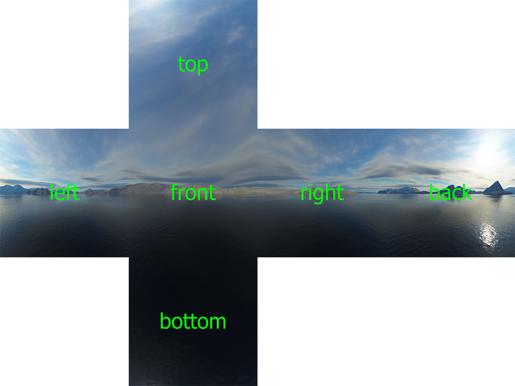
If you fold the image along the borders (bending the edges “behind the screen”), you will get a fully textured cube, inside of which a feeling of large space is created. Some resources follow this texture layout, so you will need to cut six textures for individual faces yourself. But, in most cases, they are laid out with a set of six separate images.

Here in high resolution you can download the texture for skybox, which we will use in the lesson.

Skybox loading

Since the skybox is represented as a cubic map, the loading process is not much different from what was already mentioned in the lesson. The following function is used for loading, which takes a vector with six paths to texture files:

unsigned int loadCubemap(vector faces)
{
    unsigned int textureID;
    glGenTextures(1, &textureID);
    glBindTexture(GL_TEXTURE_CUBE_MAP, textureID);
    int width, height, nrChannels;
    for (unsigned int i = 0; i < faces.size(); i++)
    {
        unsigned char *data = stbi_load(faces[i].c_str(), &width, &height, &nrChannels, 0);
        if (data)
        {
            glTexImage2D(GL_TEXTURE_CUBE_MAP_POSITIVE_X + i, 
                         0, GL_RGB, width, height, 0, GL_RGB, GL_UNSIGNED_BYTE, data
            );
            stbi_image_free(data);
        }
        else
        {
            std::cout << "Cubemap texture failed to load at path: " << faces[i] << std::endl;
            stbi_image_free(data);
        }
    }
    glTexParameteri(GL_TEXTURE_CUBE_MAP, GL_TEXTURE_MIN_FILTER, GL_LINEAR);
    glTexParameteri(GL_TEXTURE_CUBE_MAP, GL_TEXTURE_MAG_FILTER, GL_LINEAR);
    glTexParameteri(GL_TEXTURE_CUBE_MAP, GL_TEXTURE_WRAP_S, GL_CLAMP_TO_EDGE);
    glTexParameteri(GL_TEXTURE_CUBE_MAP, GL_TEXTURE_WRAP_T, GL_CLAMP_TO_EDGE);
    glTexParameteri(GL_TEXTURE_CUBE_MAP, GL_TEXTURE_WRAP_R, GL_CLAMP_TO_EDGE);
    return textureID;
}

Function code should not come as a surprise. This is all the same code for working with a cubic map that was shown in the previous section, but put together in one function.

vector faces;
{
    "right.jpg",
    "left.jpg",
    "top.jpg",
    "bottom.jpg",
    "front.jpg",
    "back.jpg"
};
unsigned int cubemapTexture = loadCubemap(faces);

Before calling the function itself, it is necessary to fill in a vector with paths to the texture files, moreover, in the order corresponding to the order of descriptions of the OpenGL enumeration elements, which describes the order of the faces of the cubic map.

Skybox display

Since we cannot do without a cube object, we will need new VAO, VBO and an array of vertices, which can be downloaded here .

Samples from a cubic map used to cover a three-dimensional cube can be made using the coordinates on the cube itself. When a cube is symmetric about the origin, then each of the coordinates of its vertices also defines a direction vector from the origin. And this direction vector is just used to select from the texture at the point corresponding to the top of the cube. As a result, we don’t even have to pass texture coordinates to the shader!
For rendering, you need a new set of shaders, quite simple. The vertex shader is trivial, only one vertex attribute is used, without texture coordinates:

#version 330 core
layout (location = 0) in vec3 aPos;
out vec3 TexCoords;
uniform mat4 projection;
uniform mat4 view;
void main()
{
    TexCoords = aPos;
    gl_Position = projection * view * vec4(aPos, 1.0);
}  

An interesting point here is that we reassign the input coordinates of the cube of the variable containing the texture coordinates for the fragment shader. The fragment shader uses them to select using samplerCube :

#version 330 core
out vec4 FragColor;
in vec3 TexCoords;
uniform samplerCube skybox;
void main()
{    
    FragColor = texture(skybox, TexCoords);
}

And this shader is pretty simple. We take the transmitted coordinates of the vertices of the cube as texture coordinates and make a selection from the cubic map.

The render also does not contain anything tricky: we attach the cubic map as the current texture and the skybox sampler immediately receives the necessary data. We will output the skybox first of all the objects in the scene, and also turn off the depth test. This ensures that the skybox is always on the background of other objects.

glDepthMask(GL_FALSE);
skyboxShader.use();
// ... задание видовой и проекционной матриц
glBindVertexArray(skyboxVAO);
glBindTexture(GL_TEXTURE_CUBE_MAP, cubemapTexture);
glDrawArrays(GL_TRIANGLES, 0, 36);
glDepthMask(GL_TRUE);
// ... вывод остальной сцены

If you try to run the program right now, you will encounter the following problem. In theory, we would like the skybox object to remain located symmetrically relative to the player’s position, no matter how far it moves - only there you can create the illusion that the environment depicted on the skybox is really huge. But the view matrix that we use applies a full set of transformations: rotation, scaling, and moving. So if the player moves, the skybox also moves! In order for the player’s actions not to affect the skybox, we should remove the movement information from the view matrix.

Perhaps you will recall the introductory lesson.in terms of coverage and the fact that we were able to get rid of the information about the movement in 4x4 matrices simply by removing the 3x3 submatrix. You can repeat this trick by simply reducing the dimension of the view matrix first to 3x3, then back to 4x4:

glm::mat4 view = glm::mat4(glm::mat3(camera.GetViewMatrix()));  

Displacement data will be deleted, but the data of the remaining transformations will be saved, which will allow the player to look around normally.

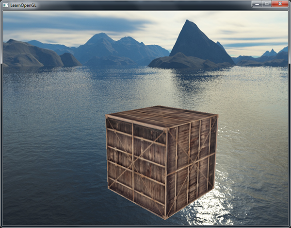
As a result, we get a picture that conveys the feeling of a large space due to skybox. Flying next to the container you will feel this sense of scale, which adds realism to the whole scene:


Try applying other texture selections and appreciate the effect that they have on the feel of the scene.

Skybox render optimization

As noted, the skybox is rendered in front of all the other objects in the scene. Works with a bang, but not too economical in resources. Judge for yourselves: when outputting in advance, we will have to execute a fragment shader for all pixels on the screen, although only some of them will remain visible in the final scene, and most could be discarded using an early depth test, saving us valuable resources.

So, for reasons of efficiency, it is worthwhile to display the skybox last. In this case, the depth buffer will be filled with the depth values ​​of all objects in the scene, and the skybox will be displayed only where the early depth test was successful, saving us the challenges of the fragment shader. But there is a catch: most likely nothing will fall into the frame, since the skybox is just a 1x1x1 cube and it will fail most of the depth tests. It is also impossible to disable the depth test before rendering, because the skybox will simply be displayed on top of the scene. You need to make the depth buffer believe that the depth of the entire skybox is 1, so that the depth test fails if there is another object in front of the skybox.

In a lesson about coordinate systemswe mentioned that perspective division is performed after the vertex shader is executed and divides the xyz components of the gl_Positions vector by the value of the w component . Also, from the depth test lesson, we know that the z component obtained after division is equal to the depth of a given vertex. Using this information, we can set the z component of the gl_Positions vector to be equal to the w component , which after perspective division will give us a depth value everywhere equal to 1:

void main()
{
    TexCoords = aPos;
    vec4 pos = projection * view * vec4(aPos, 1.0);
    gl_Position = pos.xyww;
} 

As a result, in the normalized coordinates of the device, the vertex will always have the component z = 1, which is the maximum value in the depth buffer. And the skybox will be displayed only in areas of the screen where there are no other objects (only here the depth test will be passed, since something overlaps at the other points of the skybox).

However, we will need to change the type of the depth function to GL_LEQUAL instead of the standard GL_LESS . A cleared depth buffer is filled by default with a value of 1, in the end, it is necessary to ensure that the skybox successfully passes the test for depth values ​​not strictly less than those stored in the buffer, but less than or equal.

Code using this optimization can be found here .

Environment display

So, the cubic map contains information about the environment of the scene, projected into one texture object. Such an object can be useful not only for the manufacture of skyboxes. Using a cubic map with an environment texture, you can simulate the reflective or refractive properties of objects. Such techniques using cubic maps are called environment mapping techniques and the most widely known of them are imitation of reflection and refraction.

Reflection

Reflection - the property of an object to display the surrounding space, i.e. depending on the viewing angle, the object acquires colors more or less identical to those of the surrounding environment. A mirror is an ideal example: it reflects the environment depending on the direction of the observer's gaze.

The basics of reflection physics are not too complicated. The following image shows how to find the reflection vector and use it to select from a cubic map:


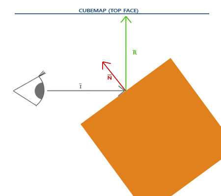
Reflection vector $$ based on gaze $$ relative to the normal vector $$. Direct calculation can be done using the built-in GLSL reflect () function . The resulting vector$$then it can be used as a direction vector to select the values ​​of the reflected color from a cubic map. As a result, the object will look like it reflects the skybox surrounding it.

Since the skybox is already prepared in our scene, creating reflections is not very difficult. Let's slightly modify the fragment shader used by the container to give it reflective properties:

#version 330 core
out vec4 FragColor;
in vec3 Normal;
in vec3 Position;
uniform vec3 cameraPos;
uniform samplerCube skybox;
void main()
{             
    vec3 I = normalize(Position - cameraPos);
    vec3 R = reflect(I, normalize(Normal));
    FragColor = vec4(texture(skybox, R).rgb, 1.0);
}

First, we calculate the direction vector of the camera (view) I and use it to calculate the reflection vector R , which is used to select from the cubic map. We again use the interpolated values Normal and Position , so we will have to clarify the vertex shader too:

#version 330 core
layout (location = 0) in vec3 aPos;
layout (location = 1) in vec3 aNormal;
out vec3 Normal;
out vec3 Position;
uniform mat4 model;
uniform mat4 view;
uniform mat4 projection;
void main()
{
    Normal = mat3(transpose(inverse(model))) * aNormal;
    Position = vec3(model * vec4(aPos, 1.0));
    gl_Position = projection * view * model * vec4(aPos, 1.0);
} 

Because normals are used again, their transformation requires the return of the use of the normal matrix. The Position vector contains the world coordinates of the vertex. It will be used in the fragment shader to compute the direction vector.

Due to the presence of normals, it is necessary to update the used array of vertex data , as well as update the code associated with the configuration of vertex attribute pointers. Also remember to set the cameraPos uniform value in each render iteration.

Before the output of the container, you should bind the cubic map object:

glBindVertexArray(cubeVAO);
glBindTexture(GL_TEXTURE_CUBE_MAP, skyboxTexture);  		
glDrawArrays(GL_TRIANGLES, 0, 36);	

As a result of the program, we get a cube leading like an ideal mirror reflecting the entire environment.


The source code is here .

When a similar special effect is assigned to the whole object, it looks like it is made of highly reflective material like polished steel or chrome. If you load the nanosuit model from the tutorial on loading models , then the whole costume will look all-metal:


It looks awesome, but in reality it is rarely which object is completely mirrored. But you can introduce reflection maps, which add some more detail to the models. Like diffuse and specular gloss maps, this type of map is a regular texture, a selection from which determines the degree of specular reflection for a fragment. With their help, it is possible to specify areas of the model that have specular reflection and its intensity. In the exercises for this lesson, you will be offered the task of adding a reflection map to the model loader developed earlier.

Refraction

Another form of imaging of the environment is refraction, which is somewhat similar to reflection. Refraction is a change in the direction of the ray of light caused by its transition through the interface between two media. It is refraction that gives the effect of changing the direction of light in liquid media, which is easily noticeable if you submerge half of your hand in water.

Refraction is described by Snell's law , in combination with a cubic map, which looks like the following:


Again we have the observation vector $$normal vector $$, and the resulting refraction vector $$. As you can see, the direction of the gaze vector is distorted due to refraction. And it is the modified vector$$will be used to select from a cubic map.

The refraction vector is easy to calculate using another built-in GLSL function - refract () , which accepts the normal vector, the direction vector of the gaze, and the ratio of the refractive indices of the adjacent materials.

The refractive index determines the degree of deviation of the direction of the beam of light following through the material. Each substance has its own coefficient, several examples are shown here:


The data from the table are used to calculate the relationship between the refractive indices of the materials through which light passes. In our case, the beam passes from air to glass (we will agree that our container is glass), which means the ratio is 1 / 1.52 = 0.658.

We have already attached the cubic map, the vertex data, including normals, are loaded, and the camera position is transferred to the corresponding uniform. It remains only to change the fragment shader:

void main()
{             
    float ratio = 1.00 / 1.52;
    vec3 I = normalize(Position - cameraPos);
    vec3 R = refract(I, normalize(Normal), ratio);
    FragColor = vec4(texture(skybox, R).rgb, 1.0);
}  

By changing the values ​​of the refractive indices, completely different visual effects can be created. When launching the application, alas, we are not waiting for a particularly impressive picture, since the glass cube does not emphasize the refraction effect too much and just looks like a cubic magnifying glass. Another thing, if you use the nanosuit model, it immediately becomes clear that the object is made of a substance similar to glass:


One can imagine that with the virtuoso application of lighting, reflection, refraction and transformation of peaks, one can achieve a very impressive simulation of the water surface.

However, it is worth noting that for physically reliable results, we need to simulate the second refraction when the beam exits from the back of the object. But for simple scenes, even simplified refraction, taking into account only one side of the object, is enough.

Changing environment maps

In this lesson, we learned how to use a combination of several images to create a skybox, which, although it looks great, does not take into account the possible presence of moving objects in the scene. Now it is imperceptible, since there is only one object in the scene. But if there was a reflecting object in the scene surrounded by other objects, we would only see the reflection of the skybox, as if there were no other objects in sight.

Using off-screen frame buffers, it is possible to create a new cubic map of the scene from the point of standing of the reflecting object by rendering the scene in six directions. Such a dynamically created cubic map could be used to create realistic reflective or refractive surfaces in which other objects are visible. This technique is called dynamic mapping of the environment, because we are preparing new cubic maps that include the entire environment, right on the fly, during the rendering process.

The approach is wonderful, but with a significant drawback - the need to render six times the entire scene for each object using a cubic map of the environment. This is a very significant blow to the performance of any application. Modern applications try to maximize the use of static skyboxes and cubed maps calculated in advance, where possible, for an approximate implementation of the dynamic display of the environment.

Despite the fact that dynamic mapping is a wonderful technique, you have to use many tricks and resourceful hacks to apply it in an application without a significant performance drawdown.

Exercises

Try adding a reflection map to the model loader created in the corresponding lesson . Nanosuit model data, including the texture of the reflection map itself, can be downloaded here . I note a few points:

• Assimp clearly does not like reflection maps in most model formats, so we cheat a bit - we will store the reflection map as a background illumination map. The map loading , accordingly, will have to be performed with the transfer of the texture type aiTextureType_AMBIENT in the material loading procedure.
• A reflection map is hastily created from a mirror gloss map. Therefore, in some places it does not fit very well on the model.
• Since the model loader already uses three texture units in the shader, you will have to use the fourth unit to bind the cubic map, since it is sampled in the same shader.

If everything is done correctly, the result will be as follows:


From a translator :

It is worth noting that when working with scans for skyboxes, you can encounter significant confusion with the orientation, especially when naming textures by the names of faces (“left”, “right”, ...), and not along the directions of the axes (+ X - positiveX, posX; -X - negativeX, negX, ...).
This is a consequence of the fact that the specification for expanding cubic maps is quite ancient and goes back to the Pixar RenderMan specification, where a cubic map uses a left-handed coordinate system and the cube itself collapses as if the observer was in the center. OpenGL itself, as we recall, uses a right-handed coordinate system.

This will have to be remembered either if the scan of the texture of interest is not the same as described here, or if there is a need to align the "sides" of the cubic map with world coordinates as if it was collapsed with an observer inside.

On the “cross” of the “cross” section shown in the “Skybox” section, the front face is considered to be such from the position of an observer located outside the cube, looking directly at it. In the code, it is loaded into the target corresponding to the positive semi-axis Z (in world coordinates). In the application, it turns out that inside the cube we observe an image mirrored along the X axis relative to what is shown on the texture.

The author himself gives a link to thisThe site where the scan used does not match the one shown in the lesson. To bring them in line, you have to swap the right and left panels, rotate the top panel clockwise by 90 °, and the bottom panel counterclockwise.


Sweeps from this site are signed according to the directions of the axes, and not the names of the faces. All that is required is to rename the files in accordance with the local table.

Understanding the essence is easier in action - in the assembled application. Sign the skybox slicing images by the alleged parties (out of curiosity, you can also add the axis of the texture coordinates) and see in the application how this will actually turn out.

PS : We have a telegram confto coordinate transfers. If you want to fit into the cycle, then you are welcome!