Frequency identification method of linear dynamic systems: theory and practice
In practical TAU applications, it is often necessary to accurately and accurately identify the control object. This article will focus on the identification of the frequency control object. This method is applicable when it is possible to physically test the control object by sinusoidal input influences by changing the frequency in a wide range. If this condition is met, then the result, as a rule, justifies the most optimistic expectations.
Let's start with a brief theoretical background. To understand the material of the article, the reader needs to have an idea of the following things:
As you know, the response of a dynamic system to a sinusoidal effect is a sinusoid with the same frequency but excellent amplitude and phase. It is these two characteristics: the amplitude and phase form the Bode graph, that is, LACH and LPC. In fact, the task of identifying a dynamic system is reduced to the experimental finding of these two graphs.
As an example, we consider the equation of a harmonic oscillator with a nonzero right-hand side as an example of a second-order linear dynamical system
Denote the Laplace transform of an arbitrary function through
  . Apply the Laplace transform to both sides of the equation
Then the characteristic equation of the dynamical system will be
A transfer function
The desired characteristics of LACH and LPCH are obtained by replacing and taking the module and function argument
  respectively
Here - amplitude (Magnitude), and
  - phase (Phase) of the corresponding component at the frequency
  . The result will be something similar to this
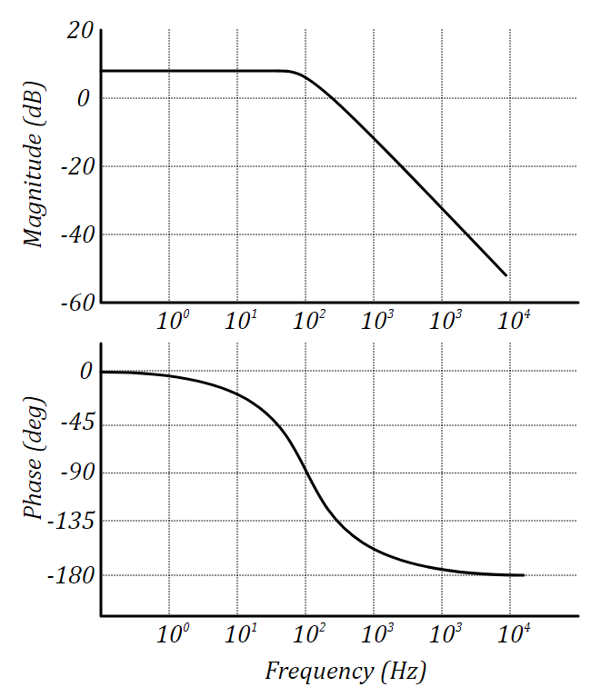
Bode characteristic: LACH and LFCH.
These two graphs unambiguously characterize a dynamic system. The converse is also true, knowing the LACH and LFC characteristics of a dynamic system with some accuracy, it is possible to completely identify this system in some confidence intervals. The question is how to get the frequency response. We will talk about this later.
By applying a sinusoidal input input, we will observe approximately the same picture.
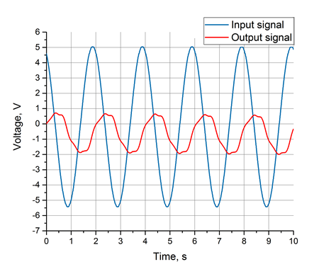
Sinusoidal input input and system response
The graph is obtained in the experiment. As can be seen from the graph, the sinusoidal component with the same frequency as the input signal is clearly present in the output signal. However, besides this, there may also be higher harmonics and noise. But do not worry, because the Fourier transform is a powerful analytical tool that is so good that it can highlight a useful signal, excluding all disturbances.
Let's say we measured two graphs, input impact and system response
  , for some given input exposure frequency
  . Both measurements must be taken synchronously and with the same sampling period.
 which must be known accurately enough. Thus, we have two sets of discrete values
 and
and  where
where  , a
, a  and
and  - values and at the corresponding discrete points in time
  . It should be noted that the total measurement time should be large enough to capture at least several (I would recommend 3 or more) periods of oscillation.
To discrete sets and
and  we can apply the discrete Fourier transform. The discrete Fourier transform converts the above signals are out of time for the second domain to the frequency, ie,
Where , a
, a  and
and  - corresponding complex amplitudes
  1st harmonics.
Now apply the discrete Fourier transform to our two signals. The figure below shows the amplitude graphs. and
and 
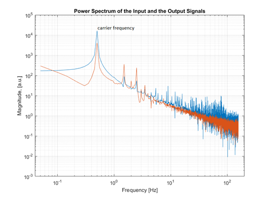
Amplitude spectrum of the input and output signal. The
graph is also obtained by processing experimental data. As you can see, a sharp peak at a frequency Hz. This is the “carrier” frequency of the input action, that is, the frequency at which the control object was excited. On both graphs, input and output, a peak is observed for this harmonic. Of the two values of complex amplitudes and at this frequency we get the value of the transfer function
  .
.
As we remember
In the case of discrete and we have
Then, on the LACH and LFC curves, we can plot the point:
What frequency does the harmonic with number have?? We answer: the harmonic frequency is given by the formula
You can also record
The expression for, in fact, the harmonic is as follows
The above procedure must be repeated a sufficient number of times to capture the entire frequency range. As a rule, you can use a larger frequency step in the low and high frequencies. Conversely, a finer step is necessary in the region of intermediate frequencies, and especially near resonances.
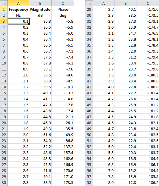
Having done such an experiment and processed the data, we obtain a table of frequency characteristics.
It is possible to immediately construct the measured graphs of LACH and LPC. It looks something like this.

LACH and LPCH, constructed from experimental data.
I must say that, although we used discrete methods, these two graphs reflect the dynamics of the originalphysical system, that is, the control object, without any simplifications associated with discretization (of course, in this frequency range).
Now you need to use MATLAB, and more specifically the System Identification Toolbox. This Toolbox has a System Identification App, an interactive application that can identify your system using frequency data. By the way, there are other options, such as, identification directly on time s m measurements.
For correct identification, you must know the order of the system. Here we will be helped by the LPCH schedule. To find out the order of the system, look at the graph of the LPF and estimate how many times the phase at a high frequency lags 90 degrees. The number of times is 90 degrees and there will be an order (denominator) of your system.
During identification, a report is automatically generated, which can be very useful. It looks like this
According to the identification report, the input data is satisfied by the found model by 92.26%. We have the following transfer function of the physical system
Now you have an object of type IDTF named tf1, with which you can do the same thing as with any other LTI System in MATLAB. In addition, the object contains information about the uncertainty of internal parameters, and if we build Bode Plot, then on the chart we can call up the display of confidence intervals. In the settings you can specify the number of standard deviations.
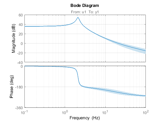
Identified model of the system with confidence intervals.
To check the correctness of identification, you can combine the experimental points with the graphs of the frequency characteristics of the identified model.
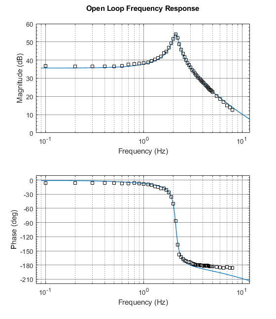
Combined graphs for LACH and LPF
Using this method greatly facilitates the process of designing a control system. The author of the article successfully developed and implemented in the LQG iron a controller for a special-purpose hydraulic circuit. In addition, this method can be used to assess the effectiveness of the control system, provided that you are physically accessible input impact on the control object from unwanted disturbances.
What you need to know
Let's start with a brief theoretical background. To understand the material of the article, the reader needs to have an idea of the following things:
- Laplace conversion
- Linear Dynamic Systems
- Characteristic equation
- Transmission function
- Discrete Fourier Transform
- Bode Feature: LACH and LFCH
Sinusoidal Response
As you know, the response of a dynamic system to a sinusoidal effect is a sinusoid with the same frequency but excellent amplitude and phase. It is these two characteristics: the amplitude and phase form the Bode graph, that is, LACH and LPC. In fact, the task of identifying a dynamic system is reduced to the experimental finding of these two graphs.
As an example, we consider the equation of a harmonic oscillator with a nonzero right-hand side as an example of a second-order linear dynamical system

Denote the Laplace transform of an arbitrary function
through . Apply the Laplace transform to both sides of the equation
Then the characteristic equation of the dynamical system will be

A transfer function

The desired characteristics of LACH and LPCH are obtained by replacing
and taking the module and function argument respectively
Here
- amplitude (Magnitude), and - phase (Phase) of the corresponding component at the frequency . The result will be something similar to this Bode characteristic: LACH and LFCH.
These two graphs unambiguously characterize a dynamic system. The converse is also true, knowing the LACH and LFC characteristics of a dynamic system with some accuracy, it is possible to completely identify this system in some confidence intervals. The question is how to get the frequency response. We will talk about this later.
By applying a sinusoidal input input, we will observe approximately the same picture.
Sinusoidal input input and system response
The graph is obtained in the experiment. As can be seen from the graph, the sinusoidal component with the same frequency as the input signal is clearly present in the output signal. However, besides this, there may also be higher harmonics and noise. But do not worry, because the Fourier transform is a powerful analytical tool that is so good that it can highlight a useful signal, excluding all disturbances.
Discrete Fourier Transform
Let's say we measured two graphs, input impact
and system response , for some given input exposure frequency . Both measurements must be taken synchronously and with the same sampling period.which must be known accurately enough. Thus, we have two sets of discrete values and where , a and - values and at the corresponding discrete points in time . It should be noted that the total measurement time should be large enough to capture at least several (I would recommend 3 or more) periods of oscillation. To discrete sets
and we can apply the discrete Fourier transform. The discrete Fourier transform converts the above signals are out of time for the second domain to the frequency, ie,
Where
, a and - corresponding complex amplitudes 1st harmonics.Method application
Now apply the discrete Fourier transform to our two signals. The figure below shows the amplitude graphs.
and Amplitude spectrum of the input and output signal. The
graph is also obtained by processing experimental data. As you can see, a sharp peak at a frequency
Hz. This is the “carrier” frequency of the input action, that is, the frequency at which the control object was excited. On both graphs, input and output, a peak is observed for this harmonic. Of the two values of complex amplitudes and at this frequency we get the value of the transfer function . As we remember

In the case of discrete
and we have
Then, on the LACH and LFC curves, we can plot the point:
What frequency does the harmonic with number have?
? We answer: the harmonic frequency is given by the formula
You can also record

The expression for, in fact, the harmonic is as follows

The above procedure must be repeated a sufficient number of times to capture the entire frequency range. As a rule, you can use a larger frequency step in the low and high frequencies. Conversely, a finer step is necessary in the region of intermediate frequencies, and especially near resonances.
Having done such an experiment and processed the data, we obtain a table of frequency characteristics.
It is possible to immediately construct the measured graphs of LACH and LPC. It looks something like this.
LACH and LPCH, constructed from experimental data.
I must say that, although we used discrete methods, these two graphs reflect the dynamics of the originalphysical system, that is, the control object, without any simplifications associated with discretization (of course, in this frequency range).
Now you need to use MATLAB, and more specifically the System Identification Toolbox. This Toolbox has a System Identification App, an interactive application that can identify your system using frequency data. By the way, there are other options, such as, identification directly on time s m measurements.
For correct identification, you must know the order of the system. Here we will be helped by the LPCH schedule. To find out the order of the system, look at the graph of the LPF and estimate how many times the phase at a high frequency lags 90 degrees. The number of times is 90 degrees and there will be an order (denominator) of your system.
During identification, a report is automatically generated, which can be very useful. It looks like this
tf1 =
  From input "u1" to output "y1":
   -97.64 s + 1.063e04
  ---------------------
  s^2 + 1.547 s + 176.7
Name: tf1
Continuous-time identified transfer function.
Parameterization:
   Number of poles: 2   Number of zeros: 1
   Number of free coefficients: 4
   Use "tfdata", "getpvec", "getcov" for parameters and their uncertainties.
Status:
Estimated using TFEST on frequency response data "h".
Fit to estimation data: 92.26% (stability enforced)
FPE: 120.6, MSE: 112.3
According to the identification report, the input data is satisfied by the found model by 92.26%. We have the following transfer function of the physical system

Now you have an object of type IDTF named tf1, with which you can do the same thing as with any other LTI System in MATLAB. In addition, the object contains information about the uncertainty of internal parameters, and if we build Bode Plot, then on the chart we can call up the display of confidence intervals. In the settings you can specify the number of standard deviations.
Identified model of the system with confidence intervals.
To check the correctness of identification, you can combine the experimental points with the graphs of the frequency characteristics of the identified model.
Combined graphs for LACH and LPF
Conclusion
Using this method greatly facilitates the process of designing a control system. The author of the article successfully developed and implemented in the LQG iron a controller for a special-purpose hydraulic circuit. In addition, this method can be used to assess the effectiveness of the control system, provided that you are physically accessible input impact on the control object from unwanted disturbances.