The book “Deep learning. Immersion in the world of neural networks "/ Blog company Publishing House" Peter "

Hi, habrozhiteli! Recently, we published the first Russian book on deep learning from Sergey Nikolenko, Arthur Kadurin and Ekaterina Arkhangelskaya. A maximum of explanations, a minimum of code, serious material about machine learning and a fascinating presentation. Now we will consider the section “Graph of computations and differentiation on it” in which the fundamental concept for the implementation of training algorithms for neural networks is introduced.

If we can imagine a complex function as a composition of simpler ones, then we can efficiently calculate its derivative with respect to any variable, which is what is required for gradient descent. The most convenient representation in the form of a composition is a representation in the form of a graph of calculations. A computation graph is a graph whose nodes are functions (usually fairly simple, taken from a pre-fixed set), and the edges connect the functions with their arguments.

It is easier to see with your own eyes than to formally define; look at pic. 2.7, which shows three graphs of calculations for the same function:


In fig. 2.7, and the graph turned out to be quite straightforward, because we allowed to use the unary function “squaring” as vertices.


And in fig. 2.7, b the graph is a little trickier: we replaced the explicit squaring by conventional multiplication. However, it didn’t increase in size because of this, because in the calculation column in Fig. 2.7, b, it is allowed to reuse the results of previous calculations several times and it is enough just to apply the same x two times to the input of the multiplication function to calculate its square. For comparison, we drew in Fig. 2.7, in the graph of the same function, but without reuse; Now it becomes a tree, but in it one has to repeat entire large subtrees, from which several paths to the root of the tree could go out at once.

In neural networks, as the basis, elementary functions of the computation graph, the functions from which the neurons are derived are usually used. For example, the scalar product of vectorsenough to build any, even the most complex neural network, composed of neurons with a function. By the way, we could express the scalar product through addition and multiplication, but it’s not necessary to “grind” too much here: any function can be elementary, for which we can easily calculate her herself and her derivative with respect to any argument. In particular, any neuron activation function, which we will discuss in detail in section 3.3, is perfect.

So, we realized that many mathematical functions, even with very complex behavior, can be represented in the form of a computation graph, where the nodes contain elementary functions, from which, like bricks, we get a complex composition, which we want to calculate. Actually, with the help of such a graph, even with a not too rich set of elementary functions, any function can be approximated arbitrarily accurately; we'll talk about this a little later.

Now back to our main subject - machine learning. As we already know, the goal of machine learning is to choose a model (most often here we mean the weight of the model specified in a parametric form) so that it best describes the data. By "best" here, as a rule, is meant the optimization of some error function. Usually it consists of the actual error on the training sample (likelihood function) and regularizers (a priori distribution), but now it’s enough for us to simply assume that there is some rather complex function that has been given to us from above, and we want to minimize it. As we already know, one of the simplest and most universal methods for optimizing complex functions is gradient descent. We also recently found out

It turns out that gradient descent and the graph of calculations are literally made for each other! As you probably were taught back in school (the school curriculum generally contains a lot of unexpectedly deep and interesting things) in order to calculate the derivative of the composition of functions (at school it was probably called the “derivative of a complex function”, as if the word “complex” weren’t enough without it values), it is enough to be able to calculate the derivatives of its components:



The rule is applied for each component separately, and the result comes out
again quite expected:


Such a partial derivative matrix is ​​called the Jacobi matrix, and its determinant is called the
Jacobian; they will meet us more than once. Now we can calculate the derivatives and gradients of any composition of functions, including vector ones, and for this we only need to be able to calculate the derivatives of each component. For a graph, all this de facto comes down to a simple but very powerful idea: if we know the computation graph and know how to take the derivative at each node, this is enough to take the derivative of the entire complex function that the graph defines!


Let’s first analyze this using an example: we’ll look at the same calculation graph, which was shown in Fig. 2.7. In fig. 2.8, and the elementary functions constituting the graph are shown; we marked each node of the graph with a new letter, from a to f, and wrote out the partial derivatives of each node for each of its inputs.

Now we can calculate the partial derivative as shown in Fig. 2.8, b: we start to calculate derivatives from the sources of the graph and use the composition differentiation formula to calculate the next derivative. For instance:


But you can go in the opposite direction, as shown in Fig. 2.8, c. In this case, we start from the source, where the partial derivative always stands, and then we expand the nodes in the reverse order by the differentiation formula of a complex function. The formula will apply here in exactly the same way; for example, in the lowest node we get:


Thus, we can apply the formula for differentiating the composition on the graph either from the sources to the sinks, getting partial derivatives of each node with the same variable 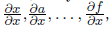or from the sinks to sources, getting the partial derivatives of sinks for all the intermediate nodes 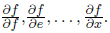Of course, in practice for machine learning we need rather, the second option than the first: the error function is usually one, and we need its partial derivatives with respect to many variables, especially for all the weights over which we want to carry out gradient descent.

In general terms, the algorithm is as follows: suppose we are given some directional acyclic computation graph G = (V, E), whose vertices are functions, and part of the vertices corresponds to the input variables x1, ..., xn and does not have incoming edges, one vertex does not have outgoing edges and corresponds to the function f (the entire graph computes this function), and the edges show the dependencies between the functions at the nodes. Then we already know how to get the function f at the “last” vertex of the graph: for this it is enough to move along the edges and calculate each function in the topological order.

And to find out the partial derivatives of this function, it is enough to move in the opposite direction. If we are interested in partial derivatives of a function, then in full accordance with the formulas above, we can calculate for each node in this way: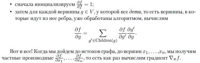


This approach is called the backpropagation, backprop, bprop algorithm, because the partial derivatives are counted in the direction opposite to the edges of the computation graph. And the algorithm for calculating the function itself or the derivative with respect to one variable, as in Fig. 2.8, b, is called forward propagation (fprop) algorithm.

And the last important note: note that for the whole time that we discussed computation graphs, differentials, gradients, and the like, we actually never seriously mentioned neural networks! Indeed, the method of calculating derivatives / gradients according to the graph of calculations in itself is completely in no way connected with neural networks. This is useful to keep in mind, especially in practical matters, which we will move on to in the next section. The fact is that the Theano and TensorFlow libraries, which we will discuss below and which make the most of deep learning, are, generally speaking, libraries for automatic differentiation, and not for training neural networks. All they do is let you set up a graph of calculations and damn efficiently, with parallelization and transfer to video cards, calculate the gradient from this graph.

Of course, on top of these libraries you can implement actually the libraries with standard neural network designs, and people do this all the time (we will consider Keras below), but it’s important not to forget the basic idea of ​​automatic differentiation. It can turn out to be much more flexible and rich than just a set of standard neural constructions, and it can happen that you will use TensorFlow extremely successfully not at all for training neural networks.

»More information about the book can be found on the publisher’s website
» Table of Contents
» Excerpt

For Khabrozhiteley 20% discount on the coupon - Deep learning