Binary Graph Search
- Transfer
Binary search is one of the most basic algorithms I know. Having a sorted list of comparable items and a target item, a binary search looks in the middle of the list and compares the value with the target item. If the goal is larger, we repeat with less than half the list, and vice versa.
For each comparison, the binary search algorithm breaks the search space in half. Thanks to this there will always be no more
 runtime comparisons
  . Beautiful, effective, useful.
 But you can always look from a different angle.
What if I try to perform a binary search on a graph? Most graph search algorithms, such as breadth-first search or depth-deep search, require linear time and were invented by pretty smart people. Therefore, if a binary search in a graph makes any sense, then it should use more information than that which conventional search algorithms have access to.
For binary search in a list, this information is the fact that the list is sorted, and to control the search, we can compare numbers with the element to be searched. But in fact, the most important information is not related to the comparability of the elements. It lies in the fact that at each stage we can get rid of half the search space. The stage “comparison with the target value” can be perceived as a black box responding to requests such as “Is this the value I was looking for?” the answers are “Yes” or “No, but look better here”
If the answers to our queries are quite useful, that is, they allow us to separate large volumes of search space at each stage, then it seems that we got a good algorithm. In fact, there is a natural graph model defined in the 2015 article by Emamjome-Zade, Kempe and Singal as follows.
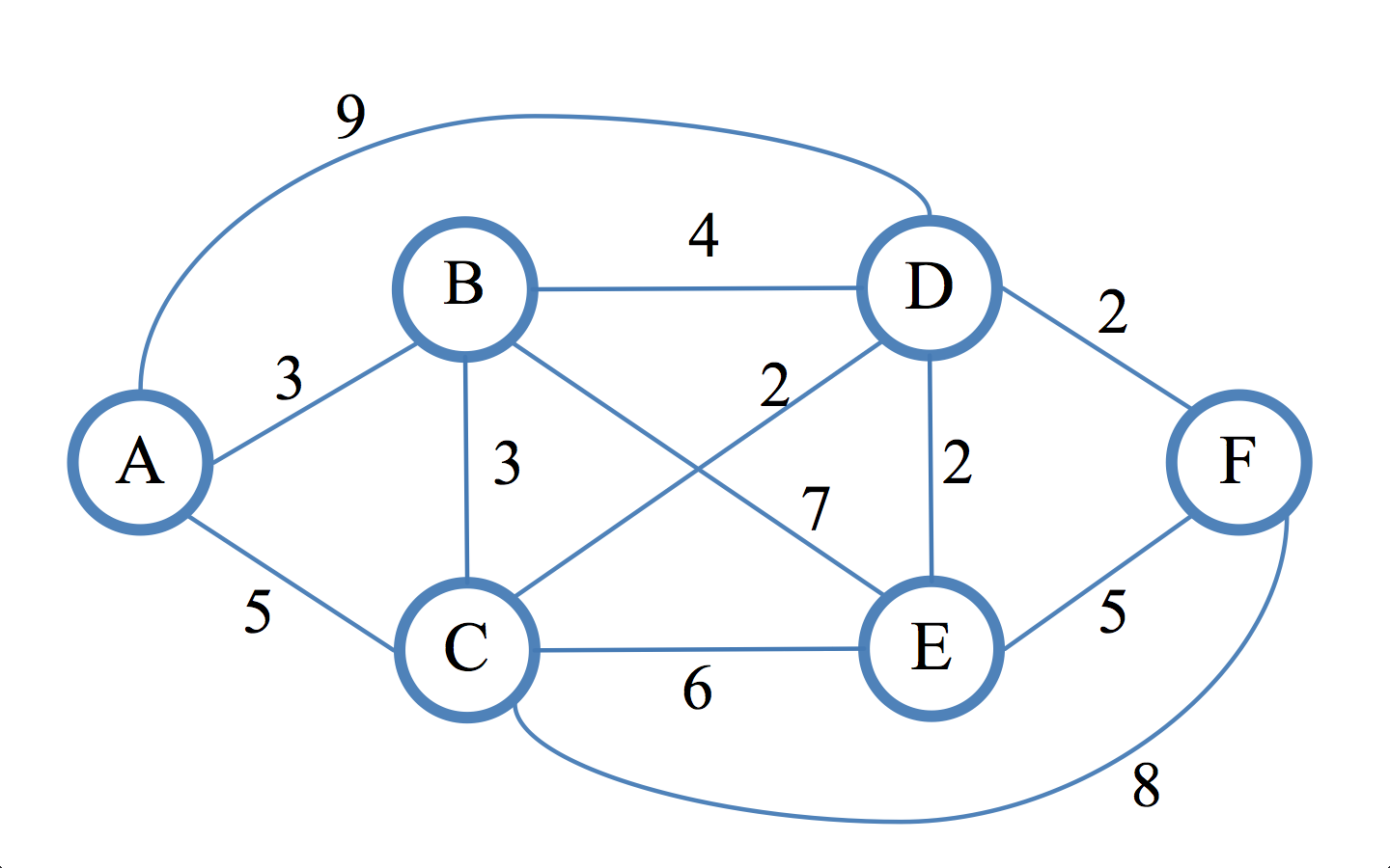
We get an undirected weighted graph as input
 with weights
  at
at  . We see the entire graph and can ask questions in the form “Is the top
 do we need? ” Answers can two options:
- Yes (we won!)
- No, but
 is an edge of on the shortest path from to the desired peak.
Our goal is to find the right peak for the minimum number of queries.
Obviously, this only works if
 is a connected graph, but small variations of the article will work for unrelated graphs. (In the general case, this is not true for directed graphs.)
 When the graph is a line, the problem is “reduced” to binary search in the sense that the same basic idea is used as in binary search: we start from the middle of the graph and the edge that we get in response to a request, tells us in which half of the graph to continue the search.
And if we make this example a little more complicated, then the generalization will become obvious:
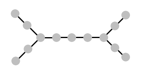
Here we start again from the “central peak” and the answer to our request will save us from one of the two halves. But how then can we choose the next vertex, because now we do not have a linear order? It should be obvious - choose the "central peak" of any half in which we find ourselves. This choice can be formalized into a rule that will work even in the absence of obvious symmetry, and as it turns out, this choice will always be correct.
Definition: median of weighted graph
relative to a subset of vertices  is the top
  (optionally located in
  ), which minimizes the sum of the distances between the vertices in >. More formally, it minimizes
Where
 - the sum of the weights of the edges along the shortest path from before
  .
. Generalizing the binary search to such a model with queries on the graph leads us to the following algorithm, which limits the search space by asking for the median at each step.
Algorithm: binary search in graphs. The graph is used as input
.- We start with many candidates
 .
. - Until we found the right peak and
 :
:- Asking for the med many and stop if we find the right vertex.
- Otherwise let will be an edge received in response to a request; calculate the set of all vertices
 for which
  is the shortest path from in
  . Call this set
 .
. - Replace on the
 .
.
- Asking for the med
- Print the only remaining vertex in
And in fact, as we will soon see, a Python implementation will be almost as simple. The most important part of the job is to compute the median and set
. Both of these operations are small varieties of Dijkstra's algorithm for calculating the shortest paths. The theorem, which is simple and well formulated by Emamjome-Zadeh and his colleagues (only about half a page on page 5), is that the algorithm requires only
 there are as many queries as in binary search.
 Before we delve into the implementation, it is worth considering a trick. Even though we are guaranteed to have no more
queries, because of our implementation of Dijkstra’s algorithm, we definitely won’t get the logarithmic algorithm. What will be useful to us in such a situation? Here we will use the “theory” - we will create a fictitious task for which we will later find application (which is used quite successfully in computer science). In this case, we will treat the query mechanism as a black box. It will be natural to imagine that requests are time consuming and are a resource that needs to be optimized. For example, as the authors wrote in an additional article, a graph can be a set of groupings of a set of data, and queries require the intervention of a person looking at the data and telling which cluster should be divided, or which two clusters should be combined. Of course, the graph is too large to process when grouping, so the median search algorithm must be implicitly defined. But the most important thing is clear: sometimes the query is the most expensive part of the algorithm.
Well, let’s realize all this! Full code, as always on Github .
We implement the algorithm
We will start with a small variation of Dijkstra's algorithm. Here we are given an “initial” point as input, and as an output we create a list of all shortest paths to all possible end vertices.
We start with a bare graph data structure.
from collections import defaultdict
from collections import namedtuple
Edge = namedtuple('Edge', ('source', 'target', 'weight'))
class Graph:
    # Голая реализация взвешенного неориентированного графа
    def __init__(self, vertices, edges=tuple()):
        self.vertices = vertices
        self.incident_edges = defaultdict(list)
        for edge in edges:
            self.add_edge(
                edge[0],
                edge[1],
                1 if len(edge) == 2 else edge[2]  # дополнительный вес
            )
    def add_edge(self, u, v, weight=1):
        self.incident_edges[u].append(Edge(u, v, weight))
        self.incident_edges[v].append(Edge(v, u, weight))
    def edge(self, u, v):
        return [e for e in self.incident_edges[u] if e.target == v][0]
Now, since most of the work in Dijkstra’s algorithm is to track the information accumulated during a graph search, we will determine the “output” data structure — a dictionary with edge weights along with back pointers to the detected shortest paths.
class DijkstraOutput:
    def __init__(self, graph, start):
        self.start = start
        self.graph = graph
        # наименьшее расстояние от начала до конечной точки v
        self.distance_from_start = {v: math.inf for v in graph.vertices}
        self.distance_from_start[start] = 0
        # список предшествующих рёбер для каждой конечной точки
        # для отслеживания списка возможного множества кратчайших путей
        self.predecessor_edges = {v: [] for v in graph.vertices}
    def found_shorter_path(self, vertex, edge, new_distance):
        # обновление решения новым найденным более коротким путём
        self.distance_from_start[vertex] = new_distance
        if new_distance < self.distance_from_start[vertex]:
            self.predecessor_edges[vertex] = [edge]
        else:  # "ничья" для нескольких кратчайших путей
            self.predecessor_edges[vertex].append(edge)
    def path_to_destination_contains_edge(self, destination, edge):
        predecessors = self.predecessor_edges[destination]
        if edge in predecessors:
            return True
        return any(self.path_to_destination_contains_edge(e.source, edge)
                   for e in predecessors)
    def sum_of_distances(self, subset=None):
        subset = subset or self.graph.vertices
        return sum(self.distance_from_start[x] for x in subset)
The real Dijkstra algorithm then performs a breadth-first search (driven by a priority queue) by
by updating metadata when finding shorter paths.def single_source_shortest_paths(graph, start):
'''
Вычисляем кратчайшие пути и расстояния от начальной вершины до всех
возможных конечных вершин. Возвращаем экземпляр DijkstraOutput.
'''
output = DijkstraOutput(graph, start)
visit_queue = [(0, start)]
while len(visit_queue) > 0:
priority, current = heapq.heappop(visit_queue)
for incident_edge in graph.incident_edges[current]:
v = incident_edge.target
weight = incident_edge.weight
distance_from_current = output.distance_from_start[current] + weight
if distance_from_current <= output.distance_from_start[v]:
output.found_shorter_path(v, incident_edge, distance_from_current)
heapq.heappush(visit_queue, (distance_from_current, v))
return outputFinally, we implement the routines for finding the median and computing
:def possible_targets(graph, start, edge):
'''
Имея заданный неориентированный граф G = (V,E), входную вершину v в V и ребро e,
инцидентное v, вычисляем множество вершин w, такое, что e находится на кратчайшем
пути от v к w.
'''
dijkstra_output = dijkstra.single_source_shortest_paths(graph, start)
return set(v for v in graph.vertices
if dijkstra_output.path_to_destination_contains_edge(v, edge))
def find_median(graph, vertices):
'''
Вычисляем в качестве output вершину во входном графе, которая минимизирует сумму
расстояний к входному множеству вершин
'''
best_dijkstra_run = min(
(single_source_shortest_paths(graph, v) for v in graph.vertices),
key=lambda run: run.sum_of_distances(vertices)
)
return best_dijkstra_run.startAnd now the core of the algorithm
QueryResult = namedtuple('QueryResult', ('found_target', 'feedback_edge'))
def binary_search(graph, query):
    '''
    Находим нужный узел в графе с помощью запросов вида "Является ли x нужной вершиной?"
    и даём ответ - или "Мы нашли нужный узел!", или "Вот ребро на кратчайшем пути к нужному узлу".
    '''
    candidate_nodes = set(x for x in graph.vertices)  # копируем
    while len(candidate_nodes) > 1:
        median = find_median(graph, candidate_nodes)
        query_result = query(median)
        if query_result.found_target:
            return median
        else:
            edge = query_result.feedback_edge
            legal_targets = possible_targets(graph, median, edge)
            candidate_nodes = candidate_nodes.intersection(legal_targets)
    return candidate_nodes.pop()
Here is an example of script execution on a sample graph that we used above in a post:
'''
Граф выглядит как дерево с равномерными весами
    a       k
     b     j
      cfghi
     d     l
    e       m
'''
G = Graph(['a', 'b', 'c', 'd', 'e', 'f', 'g', 'h', 'i',
           'j', 'k', 'l', 'm'],
          [
               ('a', 'b'),
               ('b', 'c'),
               ('c', 'd'),
               ('d', 'e'),
               ('c', 'f'),
               ('f', 'g'),
               ('g', 'h'),
               ('h', 'i'),
               ('i', 'j'),
               ('j', 'k'),
               ('i', 'l'),
               ('l', 'm'),
          ])
def simple_query(v):
    ans = input("Является ли '%s' нужной вершиной? [y/N] " % v)
    if ans and ans.lower()[0] == 'y':
        return QueryResult(True, None)
    else:
        print("Введите вершину на кратчайшем пути между"
              " '%s' и нужной вершиной. Граф: " % v)
        for w in G.incident_edges:
            print("%s: %s" % (w, G.incident_edges[w]))
        target = None
        while target not in G.vertices:
            target = input("Введите соседнюю вершину '%s': " % v)
    return QueryResult(
        False,
        G.edge(v, target)
    )
output = binary_search(G, simple_query)
print("Найдена нужная вершина: %s" % output)
The query function simply displays a reminder of the graph structure and asks the user to answer (yes / no) and report the corresponding edge, if in the case of a negative answer.
Execution Example:
Является ли 'g' нужной вершиной? [y/N] n

Введите вершину на кратчайшем пути между 'g' и нужной вершиной. Граф:

e: [Edge(source='e', target='d', weight=1)]

i: [Edge(source='i', target='h', weight=1), Edge(source='i', target='j', weight=1), Edge(source='i', target='l', weight=1)]

g: [Edge(source='g', target='f', weight=1), Edge(source='g', target='h', weight=1)]

l: [Edge(source='l', target='i', weight=1), Edge(source='l', target='m', weight=1)]

k: [Edge(source='k', target='j', weight=1)]

j: [Edge(source='j', target='i', weight=1), Edge(source='j', target='k', weight=1)]

c: [Edge(source='c', target='b', weight=1), Edge(source='c', target='d', weight=1), Edge(source='c', target='f', weight=1)]

f: [Edge(source='f', target='c', weight=1), Edge(source='f', target='g', weight=1)]

m: [Edge(source='m', target='l', weight=1)]

d: [Edge(source='d', target='c', weight=1), Edge(source='d', target='e', weight=1)]

h: [Edge(source='h', target='g', weight=1), Edge(source='h', target='i', weight=1)]

b: [Edge(source='b', target='a', weight=1), Edge(source='b', target='c', weight=1)]

a: [Edge(source='a', target='b', weight=1)]

Введите соседнюю вершину 'g': f

Является ли 'c' нужной вершиной? [y/N] n

Введите вершину на кратчайшем пути между 'c' и нужной вершиной. Граф:

[...]

Введите соседнюю вершину 'c': d

Является ли 'd' нужной вершиной? [y/N] n

Введите вершину на кратчайшем пути между 'd' и нужной вершиной. Граф:

[...]

Введите соседнюю вершину 'd': e

Найдена нужная вершина: e
Probabilistic story
The binary search we implemented in this post is pretty minimalistic. In fact, the more interesting part of Emamjome-Zade's work with colleagues is the part in which the answer to the request may be incorrect with an unknown probability.
In this case, there can be many shortest paths that are the correct answer to the request, in addition to all the incorrect answers. In particular, this excludes the strategy of transmitting the same request several times and choosing the most popular answer. If the error rate is 1/3, and there are two shortest paths to the desired vertex, then we can get a situation in which we will see three answers with equal frequency and cannot find out which one is false.
Instead, Emamjome-Zade et al. Uses a technique based on the algorithm for updating multiplicative weights (he is back in business! ) Each request gives a multiplicative increase (or decrease) for many nodes that are constant necessary vertices, provided that the answer to the request is correct. There are some more details and post-processing to avoid incredible results, but in general the main idea is as follows. Its implementation will be an excellent exercise for readers interested in deeply studying this recent article (or stretching their math muscles).
But if you look even deeper, this model of “asking and getting advice on how to improve the result” is a classic model training, first formally studied by Dana Engluin. In her model, an algorithm is designed to train the classifier. Valid queries are membership requests.and equivalence . Affiliation is, in essence, the question “What is the label of this element?”, And the equivalence query has the form “Is this a valid classifier?” If the answer is no, then an example with an incorrect label is passed.
This differs from the usual assumption of machine learning, because the learning algorithm should create an example about which he wants to get more information, and not just rely on a randomly generated subset of data. The goal is to minimize the number of queries until the algorithm exactly learns the desired hypothesis. And in fact - as we saw in this post, if we have a little extra time to study the task space, then we can create queries that receive quite a lot of information.
The binary graph search model presented here is a natural analogue of the equivalence query in the search problem: instead of a counterexample with the wrong label, we get a “push” in the right direction to the target. Pretty good!
Here we can go in different ways: (1) implement a version of the algorithm with multiplicative weights, (2) apply this technique to the ranking or grouping task, or (3) consider theoretical models of learning such as membership and equivalence in more detail.