Mathematical model of financial market dynamics
Introduction
A change in the exchange rate in the financial market affects the prices of goods and services. Therefore, it is important to know the period of time after which prices will begin to respond to changes in the exchange rate.
The difficulty of solving this problem lies in the large number of factors affecting the change in the exchange rate [1]. An effective way to weed out a number of secondary factors to determine the main market trends is to use the Wiener Hopf “white” filter [2,3].
It is clear that only the use of a filter does not solve all the problems of analyzing the impact of the exchange rate on the financial market, however, as one of the analysis tools, it is certainly interesting. In addition, using the example of such a filter, it is possible to determine the coefficients of the differential equation of the financial market.
Formulation of the problem
Based on data on fluctuations in the exchange rate using a correlation analysis and the Wiener Hopf system of equations, construct a dynamic model of the financial market with the help of which it is possible to determine the time intervals for prices to respond to changes in exchange rates.
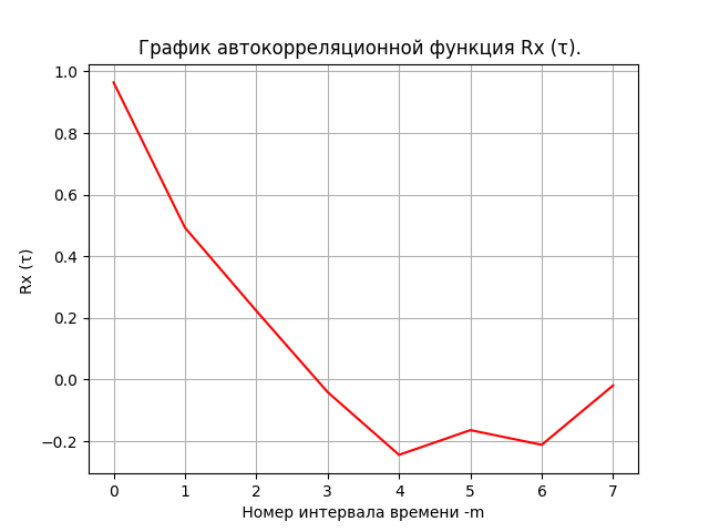
Determine the autocorrelation function Rx (τ) of the first set X of data on currency rate fluctuations and plot it
I give a listing of the solutions to this problem using Python:
import matplotlib.pyplot as plt
from sympy import *
from numpy import (zeros,arange,ones,matrix,linalg,linspace)
X=[797.17, 797.25, 797.15, 797.23, 797.15, 797.08, 797.05, 797.04, 797.14, 797.14, 797.1, 797.1, 797.11, 797.11, 797.11, 797.11, 797.11, 797.1, 797.1, 797.1, 797.12, 797.12, 797.12, 797.12, 797.12, 797.12, 797.1, 797.08]
n=len(X)
m=int(n/4)
Xsr=sum([w for w in X])/n
Dx=sum([(X[i]-Xsr)**2 for i in arange(0,n,1)])/(n-1)
Rxm=sum([(X[i]-Xsr)*(X[i+m]-Xsr) for i in arange(0,n-m,1)])/((n-m)*Dx)
def fRxm(m):
         return sum([(X[i]-Xsr)*(X[i+m]-Xsr) for i in arange(0,n-m,1)])/((n-m)*Dx)
ym=[fRxm(m) for m in arange(0,m+1)]
xm=list(arange(0,m+1,1))
M=zeros([1,m+1])
for i in arange(0,m+1,1):
         M[0,i]=fRxm(i)
plt.figure()
plt.title('График автокорреляционной функция Rx (τ). ')
plt.ylabel('Rx (τ) ')
plt.xlabel(' Номер интервала времени -m ')
plt.plot(xm, ym, 'r')
plt.grid(True)
We get:
Here
 is the time interval (offset) between the values of the random process x (t) corresponding to the value R (m) of the autocorrelation function.
 For values of Rx (τ) in the range 0.7 <= Rx (k) <= 1, the values of x (t) are statistically closely related. In other words, values that are spaced apart from each other for a period of time significantly affect each other.
For Rx (τ) values in the range 0.4 <= Rx (k) <0.7 , the x (t) values have an average statistical relationship. This means that the values are separated from each other by a period of time
 affect each other, but this influence can be predicted with a significant error.
 For values of Rx (τ) in the range 0. <= Rx (k) <0.4, the values of x (t) have a weak statistical relationship and their relationship can be neglected.
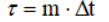
Calculate the cross-correlation function Rxy (τ) of the first data set X and the second data set Y, plot it
Here is a snippet of listing to solve this problem in Python:
Y=[577.59, 622.61, 602.23, 554.64, 567.67, 635.47, 608.27, 620.82, 561.73, 639.0, 550.1, 609.31, 640.45, 611.92, 579.33, 552.04, 597.73, 553.4, 605.72, 647.94, 602.26, 610.99, 575.95, 638.99, 631.86, 589.89, 608.17, 619.26]
n=len(Y)
m=int(n/4)
Ysr=sum([w for w in Y])/n
Dy=sum([(Y[i]-Ysr)**2 for i in arange(0,n,1)])/(n-1)
Rxy=sum([(X[i]-Xsr)*(Y[i+m]-Ysr) for i in arange(0,n-m,1)])/((n-m)*Dx**0.5*Dy**0.5)
def fRxy(m):
         return sum([(X[i]-Xsr)*(Y[i+m]-Ysr) for i in arange(0,n-m,1)])/((n-m)*Dx**0.5*Dy**0.5)
xy=[fRxy(m) for m in arange(0,m+1)]
plt.figure()
plt.title('График автокорреляционной функции Rxy (τ). ')
plt.ylabel('Rxy (τ) ')
plt.xlabel(' Номер интервала времени -m ')
plt.plot(xm, xy, 'r')
plt.grid(True)
We get:
By the maximum of the cross-correlation function Rxy , the delay or the economic lag of the market τ0 is determined . On the chart. the maximum of the function Rxy (m) corresponds to m = 4 . Consequently, a change in the exchange rate will affect the change in the price of the goods after a period of time equal to = 4 * 1 day = 4 days . That is, after three days the price of this product will change due to changes in the exchange rate of the currency (dollar).
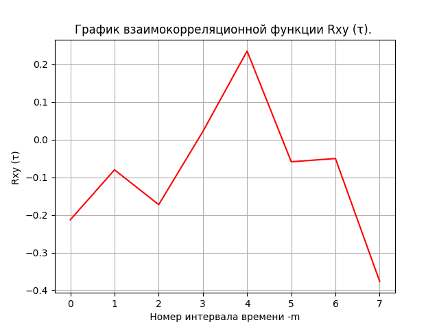
Solve the Wiener-Hopf system of equations and plot the pulse transition function h (t)
Here is a snippet of listing to solve this problem in Python:
Solving the Wiener-Hopf system of equations by the algebraic method
P=zeros([m,1])
for i in arange(0,m,1):
         P[i,0]=fRxy(i)
Q=zeros([7,7])
for i in arange(0,7,1):
         Q[0,i]=M[0,i+1]
         Q[1,i]=M[0,i]
for i in arange(0,6,1):
         Q[2,i+1]=M[0,i]
Q[2,0]=M[0,1]
for i in arange(0,5,1):
         Q[3,i+2]=M[0,i]
Q[3,1]=M[0,1]
Q[3,0]=M[0,2]
for i in arange(0,4,1):
         Q[4,i+3]=M[0,i]
Q[4,0]=M[0,3]
Q[4,1]=M[0,2]
Q[4,2]=M[0,1]
for i in arange(0,3,1):
         Q[5,i+4]=M[0,i]
Q[5,0]=M[0,4]
Q[5,1]=M[0,3]
Q[5,2]=M[0,2]
Q[5,3]=M[0,1]
for i in arange(0,2,1):
         Q[6,i+5]=M[0,i]
Q[6,0]=M[0,5]
Q[6,1]=M[0,4]
Q[6,2]=M[0,3]
Q[6,3]=M[0,2]
Q[6,4]=M[0,1]
H=linalg.solve(Q, P)
hxy=[H[m]  for m in arange(0,int(m),1)]
xm=list(arange(1,m+1,1))
plt.figure()
plt.title('График импульсной переходной функции h(t)')
plt.ylabel('H ')
plt.xlabel(' Номер интервала времени -i ')
plt.plot(xm, hxy, 'r')
plt.grid(True)
We get:
With a decrease in the exchange rate, two identical impulses and recession. For analysis, it is necessary to obtain a transition function and determine the coefficients of the differential equation of the market, the solution of which will confirm the general trend.
Construct a transition function from the found solution of the Wiener-Hopf system of equations, and obtain the differential equation of the financial market
Here is a snippet of listing to solve this problem in Python:
The construction of the transition characteristics and differential equations of the financial market
 s1=H[0,0]/2
s2=(H[0,0]+H[1,0])/2
s3=(H[1,0]+H[2,0])/2
s4=(H[2,0]+H[3,0])/2
s5=(H[3,0]+H[4,0])/2
s6=(H[4,0]+H[5,0])/2
s7=(H[5,0]+H[6,0])/2
N=zeros([8,1])
N[0,0]=0
N[1,0]=s1
N[2,0]=N[1,0]+s2
N[3,0]=N[2,0]+s3
N[4,0]=N[3,0]+s4
N[5,0]=N[4,0]+s5
N[6,0]=N[5,0]+s6
N[7,0]=N[6,0]+s7
nxy=[N[i,0] for i in arange(0,m,1)]
xm=[i for i in arange(0,m,1)]
plt.figure()
plt.plot(xm, nxy,color='r', linewidth=3, label='Решение системы Винера-Хопфа')
var('t C1 C2')
u = Function("u")(t)
de = Eq(u.diff(t, t) +0.3*u.diff(t) + u, -0.24)
print(de)
des = dsolve(de,u)
eq1=des.rhs.subs(t,0)
eq2=des.rhs.diff(t).subs(t,0)
seq=solve([eq1,eq2],C1,C2)
rez=des.rhs.subs([(C1,seq[C1]),(C2,seq[C2])])
g= lambdify(t, rez, "numpy")
t= linspace(0,7,100)
plt.title('Динамика финансового рынка')
plt.xlabel('Номер интервала (лага) времени')
plt.ylabel('y(t), N')
plt.plot(t,g(t),color='b', linewidth=3, label='Решение ДУ финансового рынка')
plt.legend(loc='best')
plt.grid(True)
plt.show()
We get:
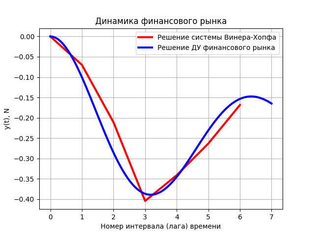
The differential equation of the financial market:
Eq (u (t) + 0.3 * Derivative (u (t), t) + Derivative (u (t), t, t), -0.24).
In the time period under consideration, the financial market can be represented by a second-order oscillatory link, corresponding to increasing periodic fluctuations in prices with increasing exchange rates and restrained periodic fluctuations in prices to depreciate.
Full listing of the program
import matplotlib.pyplot as plt
from sympy import *
from numpy import (zeros,arange,ones,matrix,linalg,linspace)
"Рассчитать автокорреляционную функцию Rx (τ) и построить ее график. "
X=[797.17, 797.25, 797.15, 797.23, 797.15, 797.08, 797.05, 797.04, 797.14, 797.14, 797.1, 797.1, 797.11, 797.11, 797.11, 797.11, 797.11, 797.1, 797.1, 797.1, 797.12, 797.12, 797.12, 797.12, 797.12, 797.12, 797.1, 797.08]
n=len(X)
m=int(n/4)
Xsr=sum([w for w in X])/n
Dx=sum([(X[i]-Xsr)**2 for i in arange(0,n,1)])/(n-1)
Rxm=sum([(X[i]-Xsr)*(X[i+m]-Xsr) for i in arange(0,n-m,1)])/((n-m)*Dx)
def fRxm(m):
         return sum([(X[i]-Xsr)*(X[i+m]-Xsr) for i in arange(0,n-m,1)])/((n-m)*Dx)
ym=[fRxm(m) for m in arange(0,m+1)]
xm=list(arange(0,m+1,1))
M=zeros([1,m+1])
for i in arange(0,m+1,1):
         M[0,i]=fRxm(i)
plt.figure()
plt.title('График автокорреляционной функция Rx (τ). ')
plt.ylabel('Rx (τ) ')
plt.xlabel(' Номер интервала времени -m ')
plt.plot(xm, ym, 'r')
plt.grid(True)
"Рассчитать взаимокорреляционную функцию Rxy (τ) первого набора X и второго набора Y данных, построить ее график"
Y=[577.59, 622.61, 602.23, 554.64, 567.67, 635.47, 608.27, 620.82, 561.73, 639.0, 550.1, 609.31, 640.45, 611.92, 579.33, 552.04, 597.73, 553.4, 605.72, 647.94, 602.26, 610.99, 575.95, 638.99, 631.86, 589.89, 608.17, 619.26]
n=len(Y)
m=int(n/4)
Ysr=sum([w for w in Y])/n
Dy=sum([(Y[i]-Ysr)**2 for i in arange(0,n,1)])/(n-1)
Rxy=sum([(X[i]-Xsr)*(Y[i+m]-Ysr) for i in arange(0,n-m,1)])/((n-m)*Dx**0.5*Dy**0.5)
def fRxy(m):
         return sum([(X[i]-Xsr)*(Y[i+m]-Ysr) for i in arange(0,n-m,1)])/((n-m)*Dx**0.5*Dy**0.5)
xy=[fRxy(m) for m in arange(0,m+1)]
plt.figure()
plt.title('График взаимокорреляционной функции Rxy (τ). ')
plt.ylabel('Rxy (τ) ')
plt.xlabel(' Номер интервала времени -m ')
plt.plot(xm, xy, 'r')
plt.grid(True)
""" Решение системы уравнений Винера-Хопфа."""
P=zeros([m,1])
for i in arange(0,m,1):
         P[i,0]=fRxy(i)
Q=zeros([7,7])
for i in arange(0,7,1):
         Q[0,i]=M[0,i+1]
         Q[1,i]=M[0,i]
for i in arange(0,6,1):
         Q[2,i+1]=M[0,i]
Q[2,0]=M[0,1]
for i in arange(0,5,1):
         Q[3,i+2]=M[0,i]
Q[3,1]=M[0,1]
Q[3,0]=M[0,2]
for i in arange(0,4,1):
         Q[4,i+3]=M[0,i]
Q[4,0]=M[0,3]
Q[4,1]=M[0,2]
Q[4,2]=M[0,1]
for i in arange(0,3,1):
         Q[5,i+4]=M[0,i]
Q[5,0]=M[0,4]
Q[5,1]=M[0,3]
Q[5,2]=M[0,2]
Q[5,3]=M[0,1]
for i in arange(0,2,1):
         Q[6,i+5]=M[0,i]
Q[6,0]=M[0,5]
Q[6,1]=M[0,4]
Q[6,2]=M[0,3]
Q[6,3]=M[0,2]
Q[6,4]=M[0,1]
H=linalg.solve(Q, P)
hxy=[H[m]  for m in arange(0,int(m),1)]
xm=list(arange(1,m+1,1))
plt.figure()
plt.title('График импульсной переходной функции h(t)')
plt.ylabel('H ')
plt.xlabel(' Номер интервала времени -i ')
plt.plot(xm, hxy, 'r')
plt.grid(True)
s1=H[0,0]/2
s2=(H[0,0]+H[1,0])/2
s3=(H[1,0]+H[2,0])/2
s4=(H[2,0]+H[3,0])/2
s5=(H[3,0]+H[4,0])/2
s6=(H[4,0]+H[5,0])/2
s7=(H[5,0]+H[6,0])/2
N=zeros([8,1])
N[0,0]=0
N[1,0]=s1
N[2,0]=N[1,0]+s2
N[3,0]=N[2,0]+s3
N[4,0]=N[3,0]+s4
N[5,0]=N[4,0]+s5
N[6,0]=N[5,0]+s6
N[7,0]=N[6,0]+s7
nxy=[N[i,0] for i in arange(0,m,1)]
xm=[i for i in arange(0,m,1)]
plt.figure()
plt.plot(xm, nxy,color='r', linewidth=3, label='Решение системы Винера-Хопфа')
var('t C1 C2')
u = Function("u")(t)
de = Eq(u.diff(t, t) +0.3*u.diff(t) +u, -0.24)
print(de)
des = dsolve(de,u)
eq1=des.rhs.subs(t,0)
eq2=des.rhs.diff(t).subs(t,0)
seq=solve([eq1,eq2],C1,C2)
rez=des.rhs.subs([(C1,seq[C1]),(C2,seq[C2])])
g= lambdify(t, rez, "numpy")
t= linspace(0,7,100)
plt.title('Динамика финансового рынка')
plt.xlabel('Номер интервала (лага) времени')
plt.ylabel('y(t), N')
plt.plot(t,g(t),color='b', linewidth=3, label='Решение ДУ финансового рынка')
plt.legend(loc='best')
plt.grid(True)
plt.show()
Conclusions:
Using the high-level programming language Python using correlation analysis and the Wiener Hopf “white” filter, an accessible tool for analyzing the dynamics of the financial market is obtained.
Thank you all for your attention!
References: