Mathematical model of a vibrating level gauge with a resonator in the form of a cantilever elliptical tube
Introduction
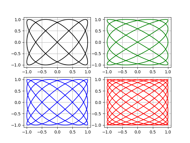
The publication [1] examined in detail the implementation in Python of a method for measuring the ratio of frequencies using Lissajous figures. As an example, the vibration forms of a cantilever elliptical tube of a vibration level gauge were analyzed [2].
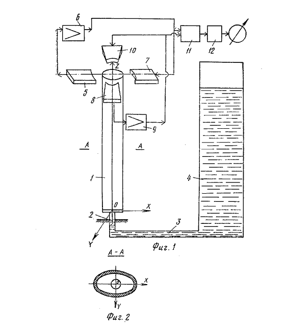
An elastically fixed tube of elliptical cross-section using self-excited systems 5,6,7 makes self-oscillations in one plane, and with the help of systems 8, 9, 10 in another plane perpendicular to the first. The tube oscillates in two mutually perpendicular planes with different frequencies close to their own. The mass of the tube depends on the level of the fluid filling it.
With a change in mass, the tube oscillation frequencies also change, which are the output signals of the level gauge. Frequencies carry additional information on the multiplicative and additive additional error compensated at frequencies processed by the microprocessor 11. The
left not resolved the question of determining the dependence of the oscillation frequency of the tube filling level of a liquid which is the subject of this publication.
Formulation of the problem
Determine the frequency of bending vibrations of the tube in two mutually perpendicular planes by the Rayleigh method using the exact equation of the bending line of the tube from the publication [1].
Using the obtained relations for the frequencies, find the dependences of sensitivity on the level and determine the ranges suitable for controlling the liquid level.
To implement these tasks using Python tools, consider two methods of solving symbolic and character-numerical. Compare these performance methods
Application of the Rayleigh method to determine the vibration frequencies of an elliptical cantilever tube
The essence of the Rayleigh method is to determine the maximum kinetic Tmax and maximum potential Pmax energies of a conservative oscillatory system, followed by equating the energies Tmax = Pmax.
From the obtained equation, one can find the oscillation frequency of the system, taking into account the fact that all harmonic components can be equated to the maximum values, for example, sin (t * w) ** 2 = 1 and cos (t * w) ** 2 = 1.
Python symbolic solution
We apply the following equation bending lines pipe:
z = (sin (k * x) -sinh (k * x) + ((cosh (k) -cos (k)) / (sin (k) -sinh (k))) * (cos (k * x) -cosh (k * x))).
We will write the following listing of the program for calculating the kinetic energy of an empty tube of length L by the function –def fp (L), on the first waveform at k = 1.875:
def fp(L):
         x,A, L, w, t, k  =symbols('x A L w t k ')
         z=(sin(k*x)-sinh(k*x)+((cosh(k) -cos(k))/(sin(k)-sinh(k)))*(cos(k*x)-cosh(k *x))).subs({k:1.875})
         dx=z*A*sin(w*t)
         dx2=(dx.diff(t))**2
         return factor(integrate(dx2,(x,0,L)))/(A**2*w**2*cos(t*w)**2)
For the kinetic energy of the liquid filling the tube to level h and oscillating with the tube as a whole, due to the small cross section, we obtain the function def fh (h):
def fh(h):
         x,A, h, w, t, k  =symbols(' x A h w t k ')
         z=(sin(k*x)-sinh(k*x)+((cosh(k) -cos(k))/(sin(k)-sinh(k)))*(cos(k*x)-cosh(k *x))).subs({k:1.875})
         dx=z*A*sin(w*t)
         dx2=(dx.diff(t))**2
         return factor(integrate (dx2,(x,0,h)))/(A**2*w**2*cos(t*w)**2)
For the potential energy of the tube, the function def pl (L) will have the form:
def pl(L):
         x,A, J, w, t, k,L  =symbols('x A J w t k L ')
         z=(sin(k*x)-sinh(k*x)+((cosh(k) -cos(k))/(sin(k)-sinh(k)))*(cos(k*x)-cosh(k *x))).subs({k:1.875})
         dx=z*A*sin(w*t)
         dx2=(dx.diff(x))**2
         return factor(integrate (dx2,(x,0,L)))/(A**2*sin(t*w)**2)
Now we can compose the Rayleigh equation –Tmax = Pmax. To do this, multiply the functions def fp (L), def fh (h), def pl (L), by the coefficients (A ** 2 * w ** 2 * cos (t * w ) ** 2) and (A ** 2 * sin (t * w) ** 2), into which they were divided in listings. Why first divide, and then multiply, I will explain later, when we consider the symbol-numerical method.
We multiply the kinetic energy functions by the mass of a unit length of a tube and a liquid - m0 and m. The potential energy function is multiplied by the stiffness E * J. Solving the Rayleigh equation for the circular frequency - w, converting it to the cyclic frequency –f = w / 2 * pi, we obtain:
f = (0.5 / pi) * ((pl (L)) * (E * J) / (m0 * fp (L) + m * fh (h))) ** 0.5
Having a function for the oscillation frequency, you can get a symbolic solution.
Character Solution Listing
from sympy import *
from numpy import arange,pi
import matplotlib.pyplot as plt
import time
start = time.time()
def fp(L):
         x,A, L, w, t, k  =symbols('x A L w t k ')
         z=(sin(k*x)-sinh(k*x)+((cosh(k) -cos(k))/(sin(k)-sinh(k)))*(cos(k*x)-cosh(k *x))).subs({k:1.875})
         dx=z*A*sin(w*t)
         dx2=(dx.diff(t))**2
         return factor(integrate(dx2,(x,0,L)))/(A**2*w**2*cos(t*w)**2)
def fh(h):
         x,A, h, w, t, k  =symbols(' x A h w t k ')
         z=(sin(k*x)-sinh(k*x)+((cosh(k) -cos(k))/(sin(k)-sinh(k)))*(cos(k*x)-cosh(k *x))).subs({k:1.875})
         dx=z*A*sin(w*t)
         dx2=(dx.diff(t))**2
         return factor(integrate (dx2,(x,0,h)))/(A**2*w**2*cos(t*w)**2)
def pl(L):
         x,A, J, w, t, k,L  =symbols('x A J w t k L ')
         z=(sin(k*x)-sinh(k*x)+((cosh(k) -cos(k))/(sin(k)-sinh(k)))*(cos(k*x)-cosh(k *x))).subs({k:1.875})
         dx=z*A*sin(w*t)
         dx2=(dx.diff(x))**2
         return factor(integrate (dx2,(x,0,L)))/(A**2*sin(t*w)**2)
""" Установка численных значений символьных переменных """
L,h,m,m0,E,J,q  =symbols(' L,h m0 m E J q ')
k1=q.subs({q:0.16})
k2=pl(L).subs({L:1})
k3=E.subs({E:196e9})*J.subs({J:2.3e-08})
k4=m0.subs({m0:1.005})
k5=m.subs({m:0.98})
k6=fp(L).subs({L:1})
"""Решения для частот чувствительностей к уровню и траекторий конца ттрубки """
x=arange(0.0,1.0,0.01)
f=k1*((k2+k3)/(k4*k6+k5*fh(h)))**0.5
y=[k1*((k2+k3)/(k4*k6+k5*fh(h).subs({h:w})))**0.5  for w in arange(0.0,1.0,0.01)]
s=f.diff(h)
y1=[s.subs({h:w}) for w in arange(0.0,1.0,0.01)]
k3=E.subs({E:196e9})*J.subs({J:1.7e-08})
f1=k1*((k2+k3)/(k4*k6+k5*fh(h)))**0.5
y2=[k1*((k2+k3)/(k4*k6+k5*fh(h).subs({h:w})))**0.5  for w in arange(0.0,1.0,0.01)]
s1=f1.diff(h)
y3=[s1.subs({h:w}) for w in arange(0.0,1.0,0.01)]
k7=fh(h).subs({h:0.7})
k3=E.subs({E:196e9})*J.subs({J:2.3e-08})
f1=k1*((k2+k3)/(k4*k6+k5*k7))**0.5
k3=E.subs({E:196e9})*J.subs({J:1.7e-08})
f2=k1*((k2+k3)/(k4*k6+k5*k7))**0.5
x1=[sin(f1*t) for t in arange(0.,2*pi,0.01)]
y4=[sin(f2*t) for t in arange(0.,2*pi,0.01)]
""" Построение графиков"""
plt.subplot(221)
plt.plot(x, y, label='f1-zox')
plt.plot(x, y2,label='f2- zoy')
plt.xlabel(' h')
plt.ylabel(' f 1,f2')
plt.legend(loc='best')
plt.grid(True)
plt.subplot(222)
plt.plot(x, y1,label='s=df/dh zox')
plt.plot(x, y3,label='s1=df1/dh - zoy')
plt.ylabel('s')
plt.xlabel(' h ')
plt.legend(loc='best')
plt.grid(True)
plt.subplot(223)
plt.plot(x1, y4,label='X,Y для h=0.7')
plt.ylabel(' Y')
plt.xlabel('X')
plt.grid(True)
plt.legend(loc='best')
stop = time.time()
print ("Время :",round(stop-start,3))
plt.show()
Result:
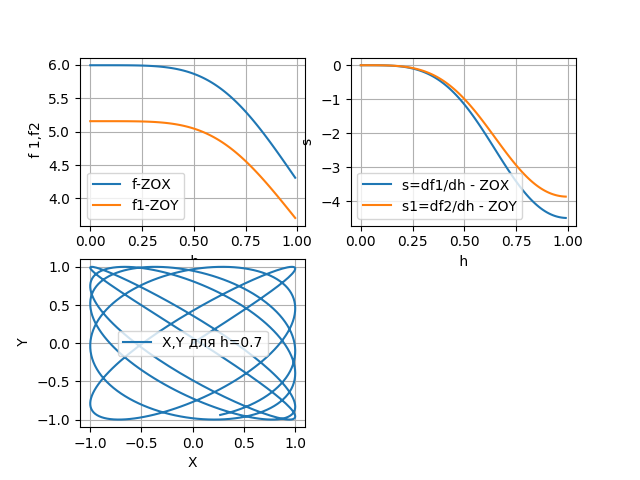
Time: 165.868
From the obtained graphs it can be seen that measurement or control can be carried out from a level of 0.75 length L tubes for aqueous solutions. The highest sensitivity at the end of the tube.
Given the high stability of the frequency of the mechanical resonator, of the order of e-6, the measurement can be carried out on a wider section from 0.5 L. And on the section from 0.75 L, microprocessor processing can be applied with compensation for both the additive and multiplicative components of the error.
Conclusion
A symbolic solution gives a good result, but takes a lot of computer time.
Python Character-Numeric Solution
We can get a symbolic solution for the functions def fp (L), def fh (h), def pl (L), so we divided them into (A ** 2 * w ** 2 * cos (t * w) ** 2 ) and (A ** 2 * sin (t * w) ** 2) to reduce the number of variables to two - L, h. And also get a symbolic solution for the sensitivity of the level gauge.
This can be done using the following listing:
Helper Listing for Character Mapping
from sympy import *
from numpy import arange,pi
import matplotlib.pyplot as plt
import time
start = time.time()
def fp(L):
         x,A, L, w, t, k  =symbols('x A L w t k ')
         z=(sin(k*x)-sinh(k*x)+((cosh(k) -cos(k))/(sin(k)-sinh(k)))*(cos(k*x)-cosh(k *x))).subs({k:1.875})
         dx=z*A*sin(w*t)
         dx2=(dx.diff(t))**2
         return factor(integrate(dx2,(x,0,L)))/(A**2*w**2*cos(t*w)**2)
def fh(h):
         x,A, h, w, t, k  =symbols(' x A h w t k ')
         z=(sin(k*x)-sinh(k*x)+((cosh(k) -cos(k))/(sin(k)-sinh(k)))*(cos(k*x)-cosh(k *x))).subs({k:1.875})
         dx=z*A*sin(w*t)
         dx2=(dx.diff(t))**2
         return factor(integrate (dx2,(x,0,h)))/(A**2*w**2*cos(t*w)**2)
def pl(L):
         x,A, J, w, t, k,L  =symbols('x A J w t k L ')
         z=(sin(k*x)-sinh(k*x)+((cosh(k) -cos(k))/(sin(k)-sinh(k)))*(cos(k*x)-cosh(k *x))).subs({k:1.875})
         dx=z*A*sin(w*t)
         dx2=(dx.diff(x))**2
         return factor(integrate (dx2,(x,0,L)))/(A**2*sin(t*w)**2)
L,h,m,m0,E,J,q  =symbols(' L,h m0 m E J q ')
f=q*((pl(L)+E*J)/(m0*fp(L)+m*fh(h)))**0.5
s=f.diff(h)
print(fp(L))
print(fh(h))
print(pl(L))
print(s)
stop = time.time()
print ("Время :",round(stop-start,3))
Time: 6.696
Listing is not loaded with multiple function calculations, therefore, its execution time is 6.696 s. Moreover, it needs to be used only once.
Now it remains to copy the results print (fp (L)), print (fh (h)), print (pl (L)), print (s) into the corresponding functions of the next listing, in which it is convenient and quick to change all the initial data for calculation. I don’t give print results, as in previous listings, so as not to clutter up the text.
Listing a character-numerical method
from numpy import (pi,cos,cosh,sin,sinh,arange)
import matplotlib.pyplot as plt
import matplotlib as mpl
mpl.rcParams['font.family'] = 'fantasy'
mpl.rcParams['font.fantasy'] = 'Comic Sans MS, Arial'
import time
start = time.time()
L=1# длинна консольной трубки в м.
d=1e-3# толщина стенки в м.
e=0.8# эксцентриситет сечения б.р.
a0=20e-3# большая внутренняя полуось в м.
a=a0+d# большая наружная полуось в м.
b0=a0*e# малая внутренняя полуось в м.
b=b0+d#малая наружная полуось в м.
E=196e9# модуль Юнга материала в н/м2.
rm=7.9e3# массовая плотность материала трубки в кг/м3.
rg=1e3#массовая плотность жидкости  в кг/м3.
J=(pi/4)*(a**3*b-a0**3*b0)# статический момент инерции по малой оси в м4.
J1=(pi/4)*(a*b**3-a0*b0**3)#статический момент инерции по большй оси в м4.
m0=pi*(a*b-a0*b0)*rm# масса единицы длинны трубки в кг/м3
m=pi*(a0*b0)*rg#масса единицы длинны жидкости в кг/м3
q=1/(2*pi)# коэффициент для перевода круговой частоты в циклическую
def fp(L):# функция кинитической энергии пустой консольной трубки L
         return (1.83012983499975*L*sin(1.875*L)**2 + 1.83012983499975*L*cos(1.875*L)**2 - 0.830129834999752*L*sinh(1.875*L)**2 + 0.830129834999752*L*cosh(1.875*L)**2 - 0.869882798951083*sin(1.875*L)**2 + 0.442735911999868*sin(1.875*L)*cos(1.875*L) + 1.73976559790217*sin(1.875*L)*sinh(1.875*L) - 1.9521384906664*sin(1.875*L)*cosh(1.875*L) - 0.885471823999735*cos(1.875*L)*sinh(1.875*L) + 0.976069245333201*sinh(1.875*L)*cosh(1.875*L) - 0.869882798951083*cosh(1.875*L)**2 + 0.869882798951083)
def fh(h):# функция кинитической энергии жидкости уровня h
          return (1.83012983499975*h*sin(1.875*h)**2 + 1.14978095631541e-15*h*sin(1.875*h)*sinh(1.875*h) + 1.83012983499975*h*cos(1.875*h)**2 - 1.07791964654569e-15*h*cos(1.875*h)*cosh(1.875*h) - 0.830129834999752*h*sinh(1.875*h)**2 + 0.830129834999752*h*cosh(1.875*h)**2 - 0.869882798951083*sin(1.875*h)**2 + 0.442735911999868*sin(1.875*h)*cos(1.875*h) + 1.73976559790217*sin(1.875*h)*sinh(1.875*h) - 1.9521384906664*sin(1.875*h)*cosh(1.875*h) - 0.885471823999735*cos(1.875*h)*sinh(1.875*h) + 0.976069245333201*sinh(1.875*h)*cosh(1.875*h) - 0.869882798951083*cosh(1.875*h)**2 + 0.869882798951083)
def pl(L):# функция потенциальной энергии консольной трубки жёсткостью E*J/L**3
         return (6.434050201171*L*sin(1.875*L)**2 + 1.48843545191282e-15*L*sin(1.875*L)*sinh(1.875*L) + 6.434050201171*L*cos(1.875*L)**2 - 2.79081647233653e-15*L*cos(1.875*L)*cosh(1.875*L) + 2.918425201171*L*sinh(1.875*L)**2 - 2.918425201171*L*cosh(1.875*L)**2 + 3.0581817150624*sin(1.875*L)**2 - 1.55649344062453*sin(1.875*L)*cos(1.875*L) + 3.11298688124907*sin(1.875*L)*cosh(1.875*L) - 6.86298688124907*cos(1.875*L)*sinh(1.875*L) + 6.1163634301248*cos(1.875*L)*cosh(1.875*L) - 3.0581817150624*sinh(1.875*L)**2 + 3.43149344062453*sinh(1.875*L)*cosh(1.875*L) - 6.1163634301248)
def f(m0,q,E,J,h,m):# чувствительность уровнимера s=df/dh
     return -0.5*m0*q*((E*J + 6.434050201171*L*sin(1.875*L)**2 + 6.434050201171*L*cos(1.875*L)**2 + 2.918425201171*L*sinh(1.875*L)**2 - 2.918425201171*L*cosh(1.875*L)**2 + 3.0581817150624*sin(1.875*L)**2 - 1.55649344062453*sin(1.875*L)*cos(1.875*L) + 3.11298688124907*sin(1.875*L)*cosh(1.875*L) - 6.86298688124907*cos(1.875*L)*sinh(1.875*L) + 6.1163634301248*cos(1.875*L)*cosh(1.875*L) - 3.0581817150624*sinh(1.875*L)**2 + 3.43149344062453*sinh(1.875*L)*cosh(1.875*L) - 6.1163634301248)/(m*(1.83012983499975*L*sin(1.875*L)**2 + 1.83012983499975*L*cos(1.875*L)**2 - 0.830129834999752*L*sinh(1.875*L)**2 + 0.830129834999752*L*cosh(1.875*L)**2 - 0.869882798951083*sin(1.875*L)**2 + 0.442735911999868*sin(1.875*L)*cos(1.875*L) + 1.73976559790217*sin(1.875*L)*sinh(1.875*L) - 1.9521384906664*sin(1.875*L)*cosh(1.875*L) - 0.885471823999735*cos(1.875*L)*sinh(1.875*L) - 0.869882798951083*sinh(1.875*L)**2 + 0.976069245333201*sinh(1.875*L)*cosh(1.875*L)) + m0*(1.83012983499975*h*sin(1.875*h)**2 + 1.83012983499975*h*cos(1.875*h)**2 - 0.830129834999752*h*sinh(1.875*h)**2 + 0.830129834999752*h*cosh(1.875*h)**2 - 0.869882798951083*sin(1.875*h)**2 + 0.442735911999868*sin(1.875*h)*cos(1.875*h) + 1.73976559790217*sin(1.875*h)*sinh(1.875*h) - 1.9521384906664*sin(1.875*h)*cosh(1.875*h) - 0.885471823999735*cos(1.875*h)*sinh(1.875*h) - 0.869882798951083*sinh(1.875*h)**2 + 0.976069245333201*sinh(1.875*h)*cosh(1.875*h))))**0.5*(1.0*sin(1.875*h)**2 - 3.26206049606656*sin(1.875*h)*cos(1.875*h) - 2.0*sin(1.875*h)*sinh(1.875*h) + 3.26206049606656*sin(1.875*h)*cosh(1.875*h) + 2.6602596699995*cos(1.875*h)**2 + 3.26206049606656*cos(1.875*h)*sinh(1.875*h) - 5.32051933999901*cos(1.875*h)*cosh(1.875*h) + 1.0*sinh(1.875*h)**2 - 3.26206049606656*sinh(1.875*h)*cosh(1.875*h) + 2.6602596699995*cosh(1.875*h)**2)/(m*(1.83012983499975*L*sin(1.875*L)**2 + 1.83012983499975*L*cos(1.875*L)**2 - 0.830129834999752*L*sinh(1.875*L)**2 + 0.830129834999752*L*cosh(1.875*L)**2 - 0.869882798951083*sin(1.875*L)**2 + 0.442735911999868*sin(1.875*L)*cos(1.875*L) + 1.73976559790217*sin(1.875*L)*sinh(1.875*L) - 1.9521384906664*sin(1.875*L)*cosh(1.875*L) - 0.885471823999735*cos(1.875*L)*sinh(1.875*L) - 0.869882798951083*sinh(1.875*L)**2 + 0.976069245333201*sinh(1.875*L)*cosh(1.875*L)) + m0*(1.83012983499975*h*sin(1.875*h)**2 + 1.83012983499975*h*cos(1.875*h)**2 - 0.830129834999752*h*sinh(1.875*h)**2 + 0.830129834999752*h*cosh(1.875*h)**2 - 0.869882798951083*sin(1.875*h)**2 + 0.442735911999868*sin(1.875*h)*cos(1.875*h) + 1.73976559790217*sin(1.875*h)*sinh(1.875*h) - 1.9521384906664*sin(1.875*h)*cosh(1.875*h) - 0.885471823999735*cos(1.875*h)*sinh(1.875*h) - 0.869882798951083*sinh(1.875*h)**2 + 0.976069245333201*sinh(1.875*h)*cosh(1.875*h)))
"""Графический анализ результатов"""
x=arange(0.0,1.0,0.01)
y1=[q*((pl(L)+E*J)/(m0*fp(L)+m*fh(h)))**0.5  for h in arange(0.0,1.0,0.01)] #числовая функция частоты трубки в сечении ZOX
J=(pi/4)*(a*b**3-a0*b0**3)#момент инерции в плоскости ZOY
y2=[q*((pl(L)+E*J)/(m0*fp(L)+m*fh(h)))**0.5  for h in arange(0.0,1.0,0.01)]#числовая функция частоты трубки в сечении ZOX
J=(pi/4)*(a**3*b-a0**3*b0)#момент инерции в плоскости ZOX
y3=[f(m0,q,E,J,h,m)  for h in arange(0.0,1.0,0.01)]#числовая функция чувствительности трубки в сечении ZOX
J=(pi/4)*(a*b**3-a0*b0**3)#момент инерции в плоскости ZOY
y4=[f(m0,q,E,J,h,m)  for h in arange(0.0,1.0,0.01)]#числовая функция чувствительности трубки в сечении ZOX
J=(pi/4)*(a**3*b-a0**3*b0)#момент инерции в плоскости ZOX
h=0.7
f1=q*((pl(L)+E*J)/(m0*fp(L)+m*fh(h)))**0.5 # частота колебаний для h=0.7 в плоскости ZOX
J=(pi/4)*(a*b**3-a0*b0**3)#момент инерции в плоскости ZOY
f2=q*((pl(L)+E*J)/(m0*fp(L)+m*fh(h)))**0.5 # частота колебаний для h=0.7 в плоскости ZOY
x1=[sin(f1*t) for t in arange(0.,2*pi,0.01)]#траектория конца трубки по Х
y5=[sin(f2*t) for t in arange(0.,2*pi,0.01)]#траектория конца трубки по Y
""" Построение графиков"""
plt.subplot(221)
plt.plot(x, y1, label='f-ZOX')
plt.plot(x, y2,label='f1-ZOY')
plt.xlabel(' h')
plt.ylabel(' f 1,f2')
plt.legend(loc='best')
plt.grid(True)
plt.subplot(222)
plt.plot(x, y3,label='s1=df1/dh - ZOX')
plt.plot(x, y4,label='s2=df2/dh - ZOY')
plt.ylabel('s')
plt.xlabel(' h ')
plt.legend(loc='best')
plt.grid(True)
plt.subplot(223)
plt.plot(x1, y5,label='X,Y для h=0.7')
plt.ylabel(' Y')
plt.xlabel('X')
plt.grid(True)
plt.legend(loc='best')
stop = time.time()
print ("Время :",round(stop-start,3))
plt.show()
Result:
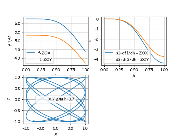
Time: 0.447
Thus, we got the same result as the symbolic method, but already 165.868 / 0.447 = 371 times faster.
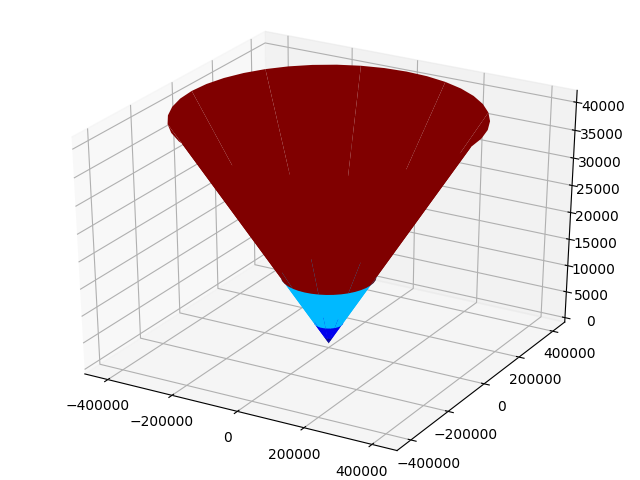
The surface on which the tube oscillates on the first form of its bending vibrations
Listing to build a surface
#!/usr/bin/env python
#coding=utf8
import pylab
import numpy
from numpy import (zeros,arange,ones,pi,sin,cos,sinh,cosh)
from matplotlib.colors import LinearSegmentedColormap
from matplotlib import cm
from mpl_toolkits.mplot3d import Axes3D
def  trubka():
         a=10;b=10;k=q[0]
         v = arange(0, 2.05*pi, 0.05*pi)
         u= zeros([len(v),1])
         for i in arange(0,len(v)):
                  u[i,0]=[sin(k*w)-sinh(k*w)+((cosh(k) -cos(k))/(sin(k)-sinh(k)))*(cos(k*w)-cosh(k *w) )for w in arange(0, 2.05*pi, 0.05*pi)][i]
         x=a*u*cos(v)
         y=b*u*sin(v)
         z=u*ones(len(v))
         return x,y,z
x,y,z=trubka()
fig = pylab.figure()
axes = Axes3D(fig)
axes.plot_surface(x, y, z, rstride=4, cstride=4, cmap = cm.jet)
pylab.show()
Result:
Conclusions:
The frequencies of bending vibrations of the tube in two mutually perpendicular planes were determined by the Rayleigh method using the exact equation of the bending line of the tube.
Using the obtained relations for frequencies, the dependences of sensitivity on the level are found and the ranges suitable for monitoring or measuring the liquid level are determined.
To implement these tasks using Python, two methods of solving symbolic and symbolic-numerical are considered. The character-numerical method runs 370 times faster than the character-based method.
References:
1. From two tuning forks from the Lissajous experiments to one elliptical level gauge tube with a step of a century and all in Python.
2. Vibration level gauge. A.S. No. 777455