Auto Encoders in Keras Part 6: VAE + GAN

Tutorial

Content

Part 1: Introduction
Part 2: Manifold learning and latent variables
Part 3: Variable Variable Encoders ( VAE )
Part 4: Conditional VAE
Part 5: GAN (Generative Adversarial Networks) and tensorflow
Part 6: VAE + GAN

In the part before last, we created a CVAE auto- encoder, the decoder of which is able to generate the number of a given label, we also tried to create pictures of the numbers of other labels in the style of a given picture. It turned out pretty well, but the numbers were generated blurry.

In the last part, we studied how GANs work , getting fairly clear images of numbers, but the ability to encode and transfer the style has disappeared.

In this part, we will try to take the best of both approaches by combining variational autoencoders ( VAE ) and generative competing networks ( GAN ).

The approach, which will be described later, is based on the article[Autoencoding beyond pixels using a learned similarity metric, Larsen et al, 2016] .

Illustration from [1]

We will examine in more detail why the restored images are blurry.

In the VAE part , the process of generating images

from latent variables was considered

.
Since the dimension of hidden variables is

much lower than the dimension of objects

(in terms of VAE, these dimensions were 2 and 784), and there is always some randomness, the same thing

can correspond to a multidimensional distribution

, that is

. This distribution can be represented as:

$P (X | Z) = f (Z) + \ epsilon,$

where is

some average most likely object for a given

, and $\ epsilon$ is the noise of some complex nature.

When we train auto-encoders, we compare the input from the sample X_s

and the output of the auto-encoder $\ tilde X_s$ using some error functionality

$L (X_s, \ tilde X_s), \\ \ tilde X_s = f_d (Z; \ theta_d), \\ Z \ sim Q (Z | X_s; \ theta_e),$

where $Q, \ f_d$ is the encoder and decoder.

By asking

, we determine the noise $\ epsilon_L$ by which we bring the real noise $\ epsilon$ .
By minimizing

, we teach the auto-encoder to adjust to the noise $\ epsilon_L$ , removing it, that is, to find the average value in a given metric (in the second part this was shown clearly with a simple artificial example).

If the noise $\ epsilon_L$ that we determine by the functional

does not correspond to the real noise $\ epsilon$ , it $f_d (Z; \ theta_2)$ will turn out to be strongly biased from the real one f (Z)

(example: if in the regression the real noise is Laplacian and the square difference is minimized, then the predicted value will be shifted towards the outliers).

Returning to the pictures: let's see how the pixel-by-pixel metric, which defines the loss in the previous parts, and the metric used by man are related. An example and illustration from [2] :

In the picture above:
(a) is the original image of the figure,
(b) is obtained from (a) by cutting a piece,
(c) is the figure (a) shifted half a pixel to the right.

In terms of the pixel-by-pixel metric (a) is much closer to (b) than to (c); although from the point of view of human perception (b) is not even a figure, but the difference between (a) and (b) is almost imperceptible.

Thus, auto encoders with pixel-by-pixel metrics smeared the image, reflecting the fact that, within close ones

the position of the numbers walks slightly in the picture,
the numbers are drawn slightly differently (although pixel by pixel it can be significantly far).

By the metric of human perception, the fact that the figure has blurred already makes it be very unlike the original. Thus, if we know a person’s metric or close to it and optimize it, then the numbers will not be blurred, and the importance of the number being complete, not like from picture (b), will increase dramatically.

You can try to manually come up with a metric that will be closer to the human. But using the GAN approach , you can train the neural network itself to look for a good metric.

About GAN'y written in the last part.

Connecting VAE and GAN

The GAN generator performs a function similar to the decoder in VAE : both samples from the prior distribution P (Z)

and translate it into P_g (X)

. However, they have different roles: the decoder restores the object encoded by the encoder, while learning, relying on some comparison metric; the generator generates a random object that can not be compared with anything, if only the discriminator could not distinguish which of the distributions

it belongs to.

Idea: add a third network to the VAE , the discriminator, and feed it the input and the restored object and the original, and train the discriminator to determine which one is which.

Illustration from [1]

Of course, use the same comparison metric fromWe can’t do VAE anymore, because by studying in it, the decoder generates images that are easily distinguishable from the original. Not to use the metric at all - either, since we would like the recreated one $\ tilde X$ to look like the original, and not just some random one P (X)

, as in a pure GAN .

But let's think about this: a discriminator, learning to distinguish a real object from a generated one, will isolate some characteristic features of one and the other. These features of the object will be encoded in the layers of the discriminator, and based on their combination, it will already give out the probability of the object being real. For example, if the image is blurry, then some neuron in the discriminator will be activated more than if it is clear. Moreover, the deeper the layer, the more abstract the characteristics of the input object are encoded in it.

Since each discriminator layer is an object description code and encodes traits that allow the discriminator to distinguish generated objects from real ones, it is possible to replace some simple metric (for example, pixel-by-pixel) with a metric over neuron activations in one of the layers:

$L (X_s, \ tilde X_s) \ longrightarrow L_d (d_l (X_s), d_l (\ tilde X_s)) \\ \ tilde X_s = f_d (Z; \ theta_d), \\ Z \ sim Q (X_s; \ theta_e) ,$

where

are the activations on the

ith layer of the discriminator, and $Q, \ f_d$ is the encoder and decoder.

At the same time, we can hope that the new metric L_d

will be better.

Below is a diagram of the resulting VAE + GAN network proposed by the authors [1] .

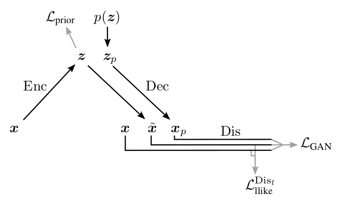
Illustration from [1]

Here:

- input object from ,
- sampled from ,
- the object generated by the decoder from ,
$\ tilde X$ - an object restored from ,
$\ mathcal L_ {prior} = KL \ left [Q (Z | X) || P (Z) \ right]$ - a loss that forces the encoder to translate to the right one for us (just like in part 3 about VAE ),
$\ mathcal L_ {llike} ^ {Dis_l} = L_d (d_l (X), d_l (\ tilde X))$ - metric between activations of the ith layer of the discriminator on the real and restored $\ tilde X = f_d (Q (X))$ ,
$\ mathcal L_ {GAN} = \ log (D (X)) + \ log (1 - D (f_d (Z))) + \ log (1 - D (f_d (Q (X))))$ - cross-entropy between the actual distribution of labels of real / generated objects, and the probability distribution of the predicted discriminator.

As with GAN , we cannot train all 3 parts of the network at the same time. The discriminator must be trained separately, in particular, it is not necessary for the discriminator to try to reduce $\ mathcal L_ {llike} ^ {Dis_l}$ , since this will collapse the activation difference by 0. Therefore, the training of all networks should be limited only to the relevant losses.

The scheme proposed by the authors:

$\ theta_ {Enc} = \ theta_ {Enc} - \ Delta _ {\ theta_ {Enc}} (\ mathcal L_ {prior} + \ mathcal L ^ {Dis_l} _ {llike}), \\ \ theta_ {Dec} = \ theta_ {Dec} - \ Delta _ {\ theta_ {Dec}} (\ gamma \ mathcal L ^ {Dis_l} _ {llike} - \ mathcal L_ {GAN}), \\ \ theta_ {Dis} = \ theta_ {Dis } - \ Delta _ {\ theta_ {Dis}} (\ mathcal L_ {GAN})$

Above you can see which networks learn which networks. Particular attention should be paid to the decoder: on the one hand, it tries to reduce the distance between the input and output in the metric of the lth layer of the discriminator ( $\ mathcal L ^ {Dis_l} _ {llike}$ ), and on the other, it tries to trick the discriminator (by increasing $\ mathcal L_ {GAN}$ ). In the article, the authors argue that by changing the coefficient $\ gamma$ , you can influence what is more important for the network: content ( $\ mathcal L ^ {Dis_l} _ {llike}$ ) or style ( $\ mathcal L_ {GAN}$ ). I cannot, however, say that I observed this effect.

Code

The code largely repeats what was in the previous parts about pure VAE and GAN .

Again, we will immediately write a conditional model.

from IPython.display import clear_output
import numpy as np
import matplotlib.pyplot as plt
%matplotlib inline
import seaborn as sns
from keras.layers import Dropout, BatchNormalization, Reshape, Flatten, RepeatVector
from keras.layers import Lambda, Dense, Input, Conv2D, MaxPool2D, UpSampling2D, concatenate
from keras.layers.advanced_activations import LeakyReLU
from keras.layers import Activation
from keras.models import Model, load_model
# Регистрация сессии в kerasfrom keras import backend as K
import tensorflow as tf
sess = tf.Session()
K.set_session(sess)
# Импорт датасетаfrom keras.datasets import mnist
from keras.utils import to_categorical
(x_train, y_train), (x_test, y_test) = mnist.load_data()
x_train = x_train.astype('float32') / 255.
x_test  = x_test .astype('float32') / 255.
x_train = np.reshape(x_train, (len(x_train), 28, 28, 1))
x_test  = np.reshape(x_test,  (len(x_test),  28, 28, 1))
y_train_cat = to_categorical(y_train).astype(np.float32)
y_test_cat  = to_categorical(y_test).astype(np.float32)
# Глобальные константы
batch_size = 64
batch_shape = (batch_size, 28, 28, 1)
latent_dim = 8
num_classes = 10
dropout_rate = 0.3
gamma = 1# Коэффициент гамма# Итераторы тренировочных и тестовых батчейdefgen_batch(x, y):
    n_batches = x.shape[0] // batch_size
    while(True):
        idxs = np.random.permutation(y.shape[0])
        x = x[idxs]
        y = y[idxs]
        for i in range(n_batches):
            yield x[batch_size*i: batch_size*(i+1)], y[batch_size*i: batch_size*(i+1)]
train_batches_it = gen_batch(x_train, y_train_cat)
test_batches_it  = gen_batch(x_test,  y_test_cat)
# Входные плейсхолдеры
x_ = tf.placeholder(tf.float32, shape=(None, 28, 28, 1),  name='image')
y_ = tf.placeholder(tf.float32, shape=(None, 10),         name='labels')
z_ = tf.placeholder(tf.float32, shape=(None, latent_dim), name='z')
img = Input(tensor=x_)
lbl = Input(tensor=y_)
z   = Input(tensor=z_)

The description of models from GAN differs almost only in the added encoder.

defadd_units_to_conv2d(conv2, units):
    dim1 = int(conv2.shape[1])
    dim2 = int(conv2.shape[2])
    dimc = int(units.shape[1])
    repeat_n = dim1*dim2
    units_repeat = RepeatVector(repeat_n)(lbl)
    units_repeat = Reshape((dim1, dim2, dimc))(units_repeat)
    return concatenate([conv2, units_repeat])
# у меня получалось, что батч-нормализация очень сильно тормозит обучение на начальных этапах (подозреваю, что из-за того, что P и P_g почти не ра)defapply_bn_relu_and_dropout(x, bn=False, relu=True, dropout=True):if bn:
        x = BatchNormalization(momentum=0.99, scale=False)(x)
    if relu:
        x = LeakyReLU()(x)
    if dropout:
        x = Dropout(dropout_rate)(x)
    return x
with tf.variable_scope('encoder'):
    x = Conv2D(32, kernel_size=(3, 3), strides=(2, 2), padding='same')(img)
    x = apply_bn_relu_and_dropout(x)
    x = MaxPool2D((2, 2), padding='same')(x)
    x = Conv2D(64, kernel_size=(3, 3), padding='same')(x)
    x = apply_bn_relu_and_dropout(x)
    x = Flatten()(x)
    x = concatenate([x, lbl])
    h = Dense(64)(x)
    h = apply_bn_relu_and_dropout(h)
    z_mean    = Dense(latent_dim)(h)
    z_log_var = Dense(latent_dim)(h)
    defsampling(args):
        z_mean, z_log_var = args
        epsilon = K.random_normal(shape=(batch_size, latent_dim), mean=0., stddev=1.0)
        return z_mean + K.exp(K.clip(z_log_var/2, -2, 2)) * epsilon
    l = Lambda(sampling, output_shape=(latent_dim,))([z_mean, z_log_var])
encoder = Model([img, lbl], [z_mean, z_log_var, l], name='Encoder')
with tf.variable_scope('decoder'):
    x = concatenate([z, lbl])
    x = Dense(7*7*128)(x)
    x = apply_bn_relu_and_dropout(x)
    x = Reshape((7, 7, 128))(x)
    x = UpSampling2D(size=(2, 2))(x)
    x = Conv2D(64, kernel_size=(5, 5), padding='same')(x)
    x = apply_bn_relu_and_dropout(x)
    x = Conv2D(32, kernel_size=(3, 3), padding='same')(x)
    x = UpSampling2D(size=(2, 2))(x)
    x = apply_bn_relu_and_dropout(x)
    decoded = Conv2D(1, kernel_size=(5, 5), activation='sigmoid', padding='same')(x)
decoder = Model([z, lbl], decoded, name='Decoder')
with tf.variable_scope('discrim'):
    x = Conv2D(128, kernel_size=(7, 7), strides=(2, 2), padding='same')(img)
    x = MaxPool2D((2, 2), padding='same')(x)
    x = apply_bn_relu_and_dropout(x)
    x = add_units_to_conv2d(x, lbl)
    x = Conv2D(64, kernel_size=(3, 3), padding='same')(x)
    x = MaxPool2D((2, 2), padding='same')(x)
    x = apply_bn_relu_and_dropout(x)
    # l-слой на котором будем сравнивать активации
    l = Conv2D(16, kernel_size=(3, 3), padding='same')(x)
    x = apply_bn_relu_and_dropout(x)
    h = Flatten()(x)
    d = Dense(1, activation='sigmoid')(h)
discrim = Model([img, lbl], [d, l], name='Discriminator')

Building a graph of calculations based on models:

z_mean, z_log_var, encoded_img = encoder([img, lbl])
decoded_img = decoder([encoded_img, lbl])
decoded_z   = decoder([z,           lbl])
discr_img,     discr_l_img     = discrim([img,         lbl])
discr_dec_img, discr_l_dec_img = discrim([decoded_img, lbl])
discr_dec_z,   discr_l_dec_z   = discrim([decoded_z,   lbl])
cvae_model = Model([img, lbl], decoder([encoded_img, lbl]), name='cvae')
cvae =  cvae_model([img, lbl])

Definition of losses:

It is interesting that the result was slightly better if, as a metric on layer activations, we did not take MSE , but cross-entropy.

# Базовые лоссы
L_prior = -0.5*tf.reduce_sum(1. + tf.clip_by_value(z_log_var, -2, 2) - tf.square(z_mean) - tf.exp(tf.clip_by_value(z_log_var, -2, 2)))/28/28
log_dis_img     = tf.log(discr_img + 1e-10)
log_dis_dec_z   = tf.log(1. - discr_dec_z + 1e-10)
log_dis_dec_img = tf.log(1. - discr_dec_img + 1e-10)
L_GAN = -1/4*tf.reduce_sum(log_dis_img + 2*log_dis_dec_z + log_dis_dec_img)/28/28# L_dis_llike = tf.reduce_sum(tf.square(discr_l_img - discr_l_dec_img))/28/28
L_dis_llike = tf.reduce_sum(tf.nn.sigmoid_cross_entropy_with_logits(labels=tf.sigmoid(discr_l_img),
                                                                    logits=discr_l_dec_img))/28/28# Лоссы энкодера, декодера, дискриминатора
L_enc = L_dis_llike + L_prior 
L_dec = gamma * L_dis_llike - L_GAN
L_dis = L_GAN
# Определение шагов оптимизатора
optimizer_enc = tf.train.RMSPropOptimizer(0.001)
optimizer_dec = tf.train.RMSPropOptimizer(0.0003)
optimizer_dis = tf.train.RMSPropOptimizer(0.001)
encoder_vars = tf.get_collection(tf.GraphKeys.TRAINABLE_VARIABLES, "encoder")
decoder_vars = tf.get_collection(tf.GraphKeys.TRAINABLE_VARIABLES, "decoder")
discrim_vars = tf.get_collection(tf.GraphKeys.TRAINABLE_VARIABLES, "discrim")
step_enc = optimizer_enc.minimize(L_enc, var_list=encoder_vars)
step_dec = optimizer_dec.minimize(L_dec, var_list=decoder_vars)
step_dis = optimizer_dis.minimize(L_dis, var_list=discrim_vars)
defstep(image, label, zp):
    l_prior, dec_image, l_dis_llike, l_gan, _, _ = sess.run([L_prior, decoded_z, L_dis_llike, L_GAN, step_enc, step_dec],
                                                            feed_dict={z:zp, img:image, lbl:label, K.learning_phase():1})
    return l_prior, dec_image, l_dis_llike, l_gan
defstep_d(image, label, zp):
    l_gan, _ = sess.run([L_GAN, step_dis], feed_dict={z:zp, img:image, lbl:label, K.learning_phase():1})
    return l_gan

Functions for drawing pictures after and during training:

Code

digit_size = 28defplot_digits(*args, invert_colors=False):
    args = [x.squeeze() for x in args]
    n = min([x.shape[0] for x in args])
    figure = np.zeros((digit_size * len(args), digit_size * n))
    for i in range(n):
        for j in range(len(args)):
            figure[j * digit_size: (j + 1) * digit_size,
                   i * digit_size: (i + 1) * digit_size] = args[j][i].squeeze()
    if invert_colors:
        figure = 1-figure
    plt.figure(figsize=(2*n, 2*len(args)))
    plt.imshow(figure, cmap='Greys_r')
    plt.grid(False)
    ax = plt.gca()
    ax.get_xaxis().set_visible(False)
    ax.get_yaxis().set_visible(False)
    plt.show()
# Массивы, в которые будем сохранять результаты, для последующей визуализации
figs = [[] for x in range(num_classes)]
periods = []
save_periods = list(range(100)) + list(range(100, 1000, 10))
n = 15# Картинка с 15x15 цифрfrom scipy.stats import norm
# Так как сэмплируем из N(0, I), то сетку узлов, в которых генерируем цифры берем из обратной функции распределения
grid_x = norm.ppf(np.linspace(0.05, 0.95, n))
grid_y = norm.ppf(np.linspace(0.05, 0.95, n))
grid_y = norm.ppf(np.linspace(0.05, 0.95, n))
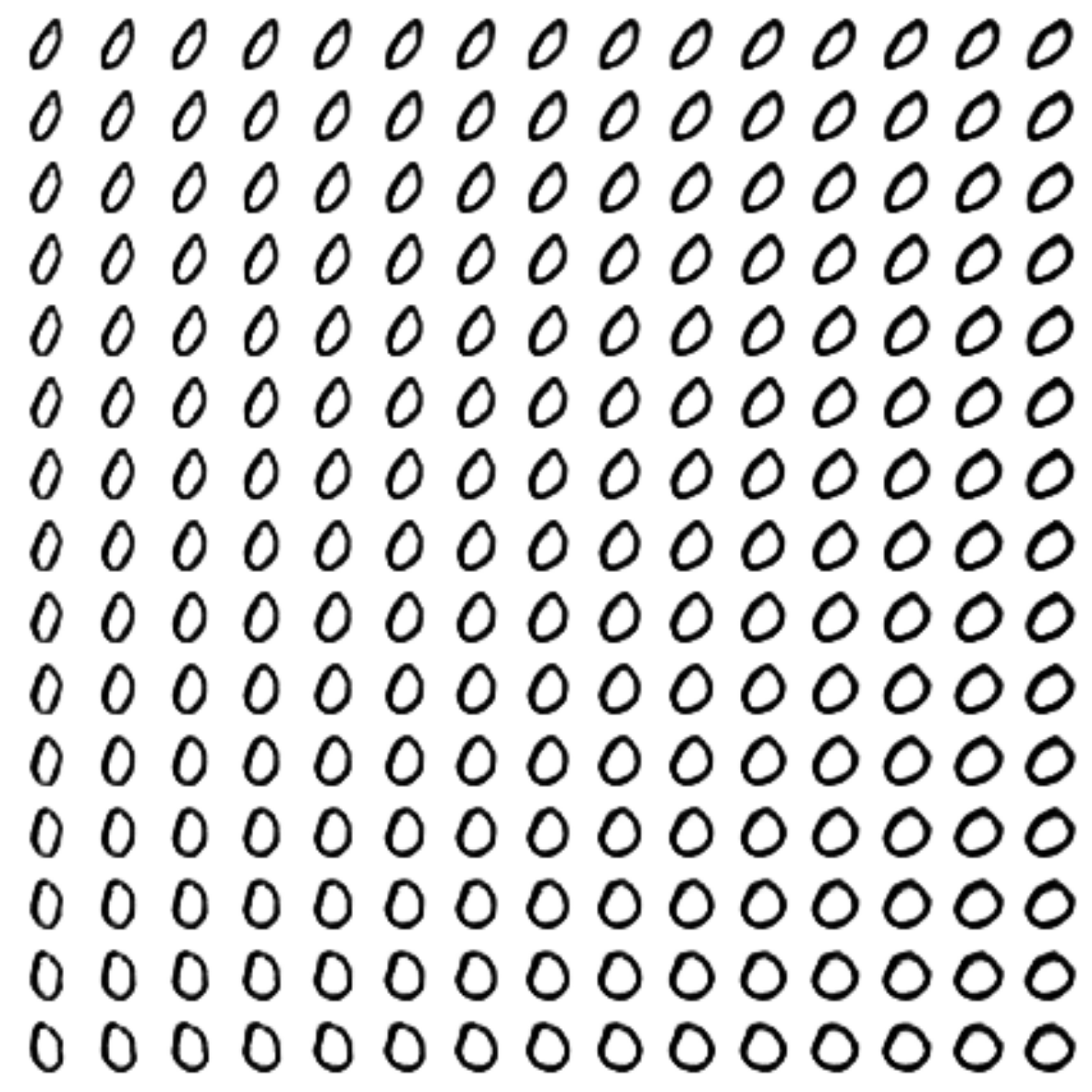
defdraw_manifold(label, show=True):# Рисование цифр из многообразия
    figure = np.zeros((digit_size * n, digit_size * n))
    input_lbl = np.zeros((1, 10))
    input_lbl[0, label] = 1for i, yi in enumerate(grid_x):
        for j, xi in enumerate(grid_y):
            z_sample = np.zeros((1, latent_dim))
            z_sample[:, :2] = np.array([[xi, yi]])
            x_decoded = sess.run(decoded_z, feed_dict={z:z_sample, lbl:input_lbl, K.learning_phase():0})
            digit = x_decoded[0].squeeze()
            figure[i * digit_size: (i + 1) * digit_size,
                   j * digit_size: (j + 1) * digit_size] = digit
    if show:
        # Визуализация
        plt.figure(figsize=(15, 15))
        plt.imshow(figure, cmap='Greys')
        plt.grid(False)
        ax = plt.gca()
        ax.get_xaxis().set_visible(False)
        ax.get_yaxis().set_visible(False)
        plt.show()
    return figure
# Рисование распределения zdefdraw_z_distr(z_predicted):
    im = plt.scatter(z_predicted[:, 0], z_predicted[:, 1])
    im.axes.set_xlim(-5, 5)
    im.axes.set_ylim(-5, 5)
    plt.show()
defon_n_period(period):
    n_compare = 10
    clear_output() # Не захламляем output# Сравнение реальных и декодированных цифр
    b = next(test_batches_it)
    decoded = sess.run(cvae, feed_dict={img:b[0], lbl:b[1], K.learning_phase():0})
    plot_digits(b[0][:n_compare], decoded[:n_compare])
    # Рисование многообразия для рандомного y
    draw_lbl = np.random.randint(0, num_classes)    
    print(draw_lbl)
    for label in range(num_classes):
        figs[label].append(draw_manifold(label, show=label==draw_lbl))
    xs = x_test[y_test == draw_lbl]
    ys = y_test_cat[y_test == draw_lbl]
    z_predicted = sess.run(z_mean, feed_dict={img:xs, lbl:ys, K.learning_phase():0})
    draw_z_distr(z_predicted)
    periods.append(period)

Learning process:

sess.run(tf.global_variables_initializer())
nb_step = 3# Количество шагов во внутреннем цикле
batches_per_period = 3for i in range(48000):
    print('.', end='')
    # Шаги обучения дискриминатораfor j in range(nb_step):
        b0, b1 = next(train_batches_it)
        zp = np.random.randn(batch_size, latent_dim)
        l_g = step_d(b0, b1, zp)
        if l_g < 1.0:
            break# Шаг обучения декодера и энкодераfor j in range(nb_step):
        l_p, zx, l_d, l_g = step(b0, b1, zp)
        if l_g > 0.4:
            break
        b0, b1 = next(train_batches_it)
        zp = np.random.randn(batch_size, latent_dim)
    # Периодическая визуализация результатаifnot i % batches_per_period:
        period = i // batches_per_period
        if period in save_periods:
            on_n_period(period)
        print(i, l_p, l_d, l_g)

GIF Drawing Function:

Code

from matplotlib.animation import FuncAnimation
from matplotlib import cm
import matplotlib
defmake_2d_figs_gif(figs, periods, c, fname, fig, batches_per_period): 
    norm = matplotlib.colors.Normalize(vmin=0, vmax=1, clip=False)
    im = plt.imshow(np.zeros((28,28)), cmap='Greys', norm=norm)
    plt.grid(None)
    plt.title("Label: {}\nBatch: {}".format(c, 0))
    defupdate(i):
        im.set_array(figs[i])
        im.axes.set_title("Label: {}\nBatch: {}".format(c, periods[i]*batches_per_period))
        im.axes.get_xaxis().set_visible(False)
        im.axes.get_yaxis().set_visible(False)
        return im
    anim = FuncAnimation(fig, update, frames=range(len(figs)), interval=100)
    anim.save(fname, dpi=80, writer='ffmpeg')
for label in range(num_classes):
    make_2d_figs_gif(figs[label], periods, label, "./figs6/manifold_{}.mp4".format(label), plt.figure(figsize=(10,10)), batches_per_period)

Since we again have a model based on an auto-encoder, we can apply style transfer:

Code

# Трансфер стиляdefstyle_transfer(X, lbl_in, lbl_out):
    rows = X.shape[0]
    if isinstance(lbl_in, int):
        label = lbl_in
        lbl_in = np.zeros((rows, 10))
        lbl_in[:, label] = 1if isinstance(lbl_out, int):
        label = lbl_out
        lbl_out = np.zeros((rows, 10))
        lbl_out[:, label] = 1# Кодирем стиль входящего изображения
    zp = sess.run(z_mean, feed_dict={img:X, lbl:lbl_in, K.learning_phase():0})
    # Восстанавливаем из этого стиля, заменяя лейбл
    created = sess.run(decoded_z, feed_dict={z:zp, lbl:lbl_out, K.learning_phase():0})
    return created
# Картинка трансфера стиляdefdraw_random_style_transfer(label):
    n = 10
    generated = []
    idxs = np.random.permutation(y_test.shape[0])
    x_test_permut = x_test[idxs]
    y_test_permut = y_test[idxs]
    prot = x_test_permut[y_test_permut == label][:batch_size]
    for i in range(num_classes):
        generated.append(style_transfer(prot, label, i)[:n])
    generated[label] = prot
    plot_digits(*generated, invert_colors=True)
draw_random_style_transfer(7)

results

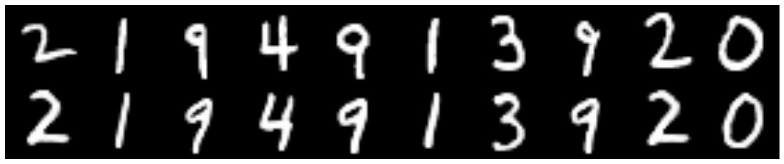
Comparison with simple CVAE

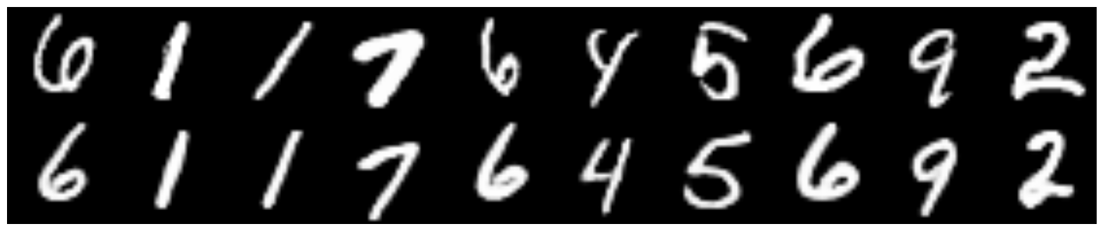
Above are the originals of the numbers, from the bottom restored.

CVAE , hidden dimension - 2

CVAE + GAN , hidden dimension - 2

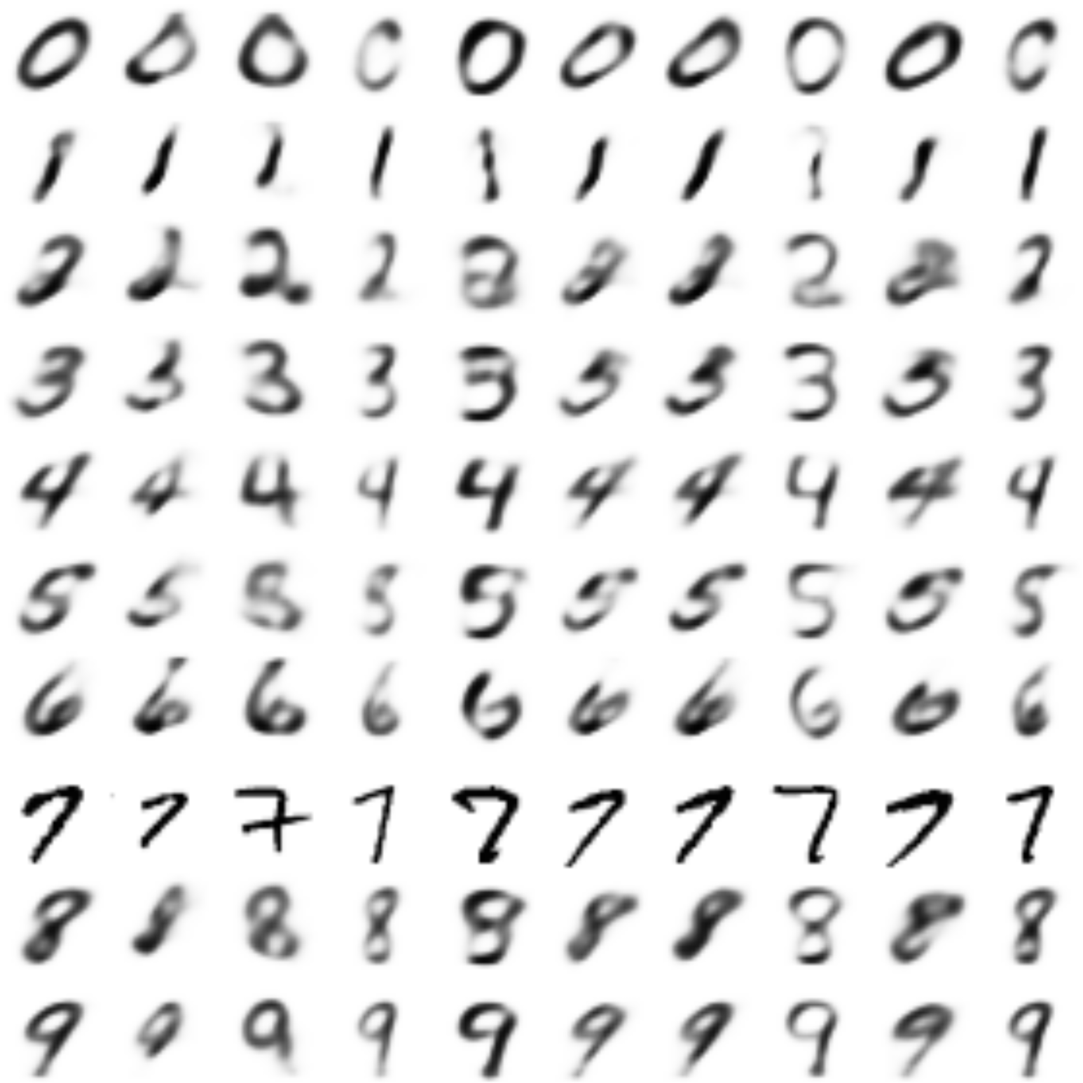
CVAE + GAN , hidden dimension - 8

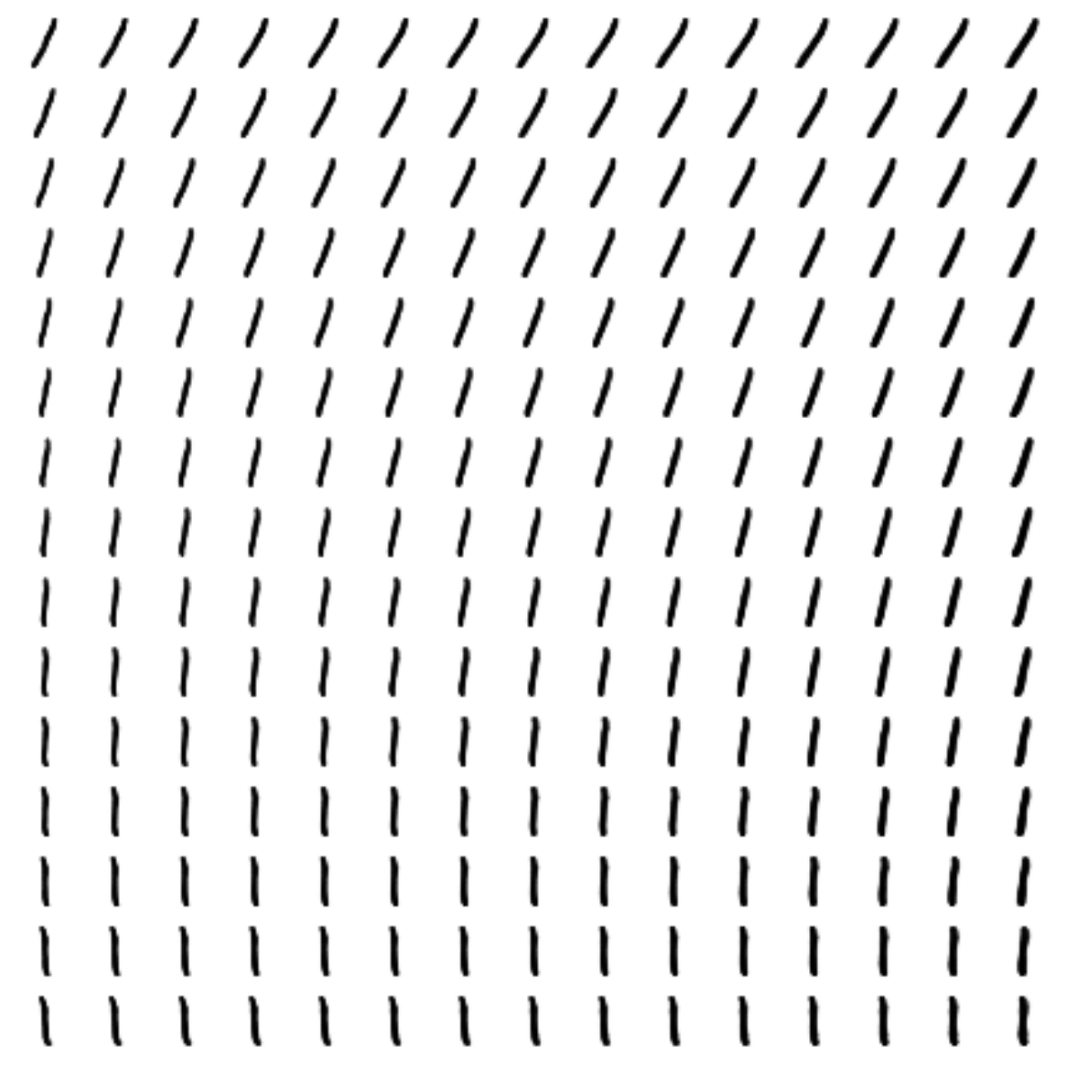
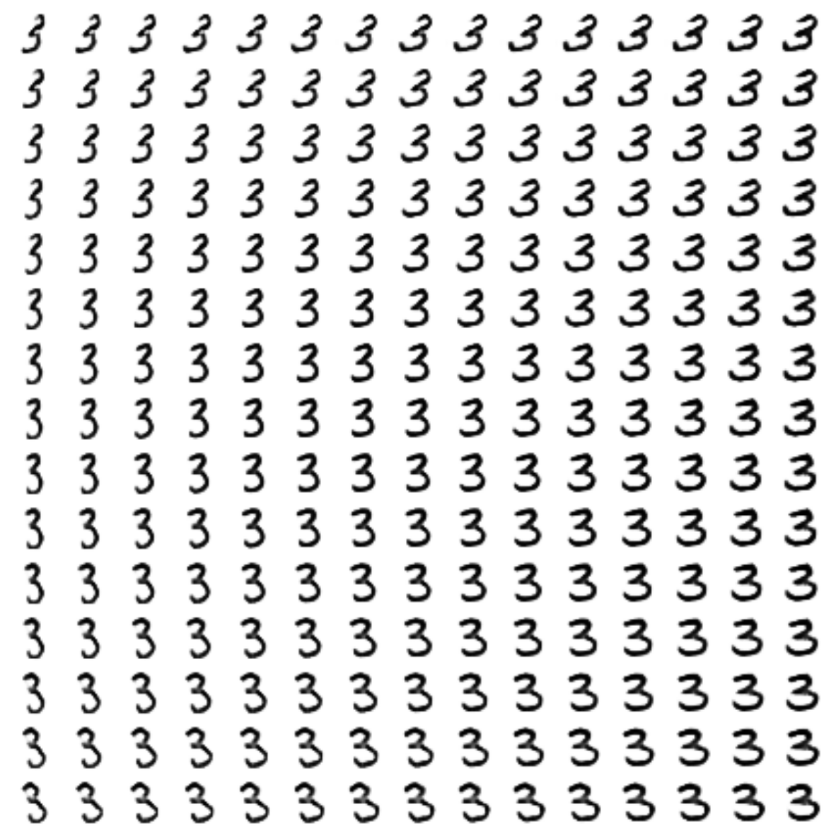
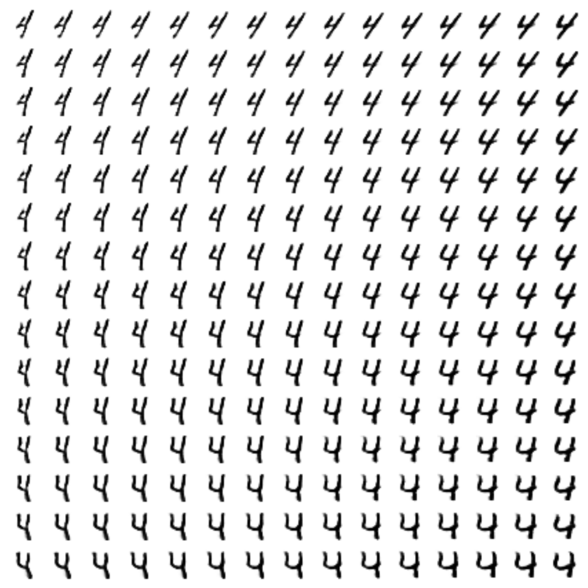
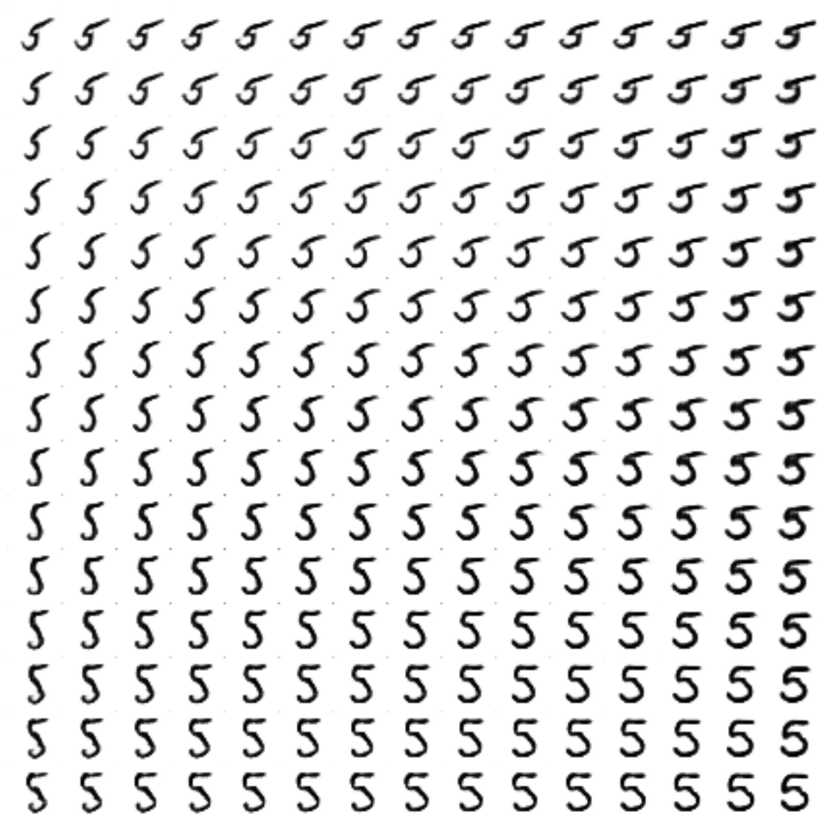
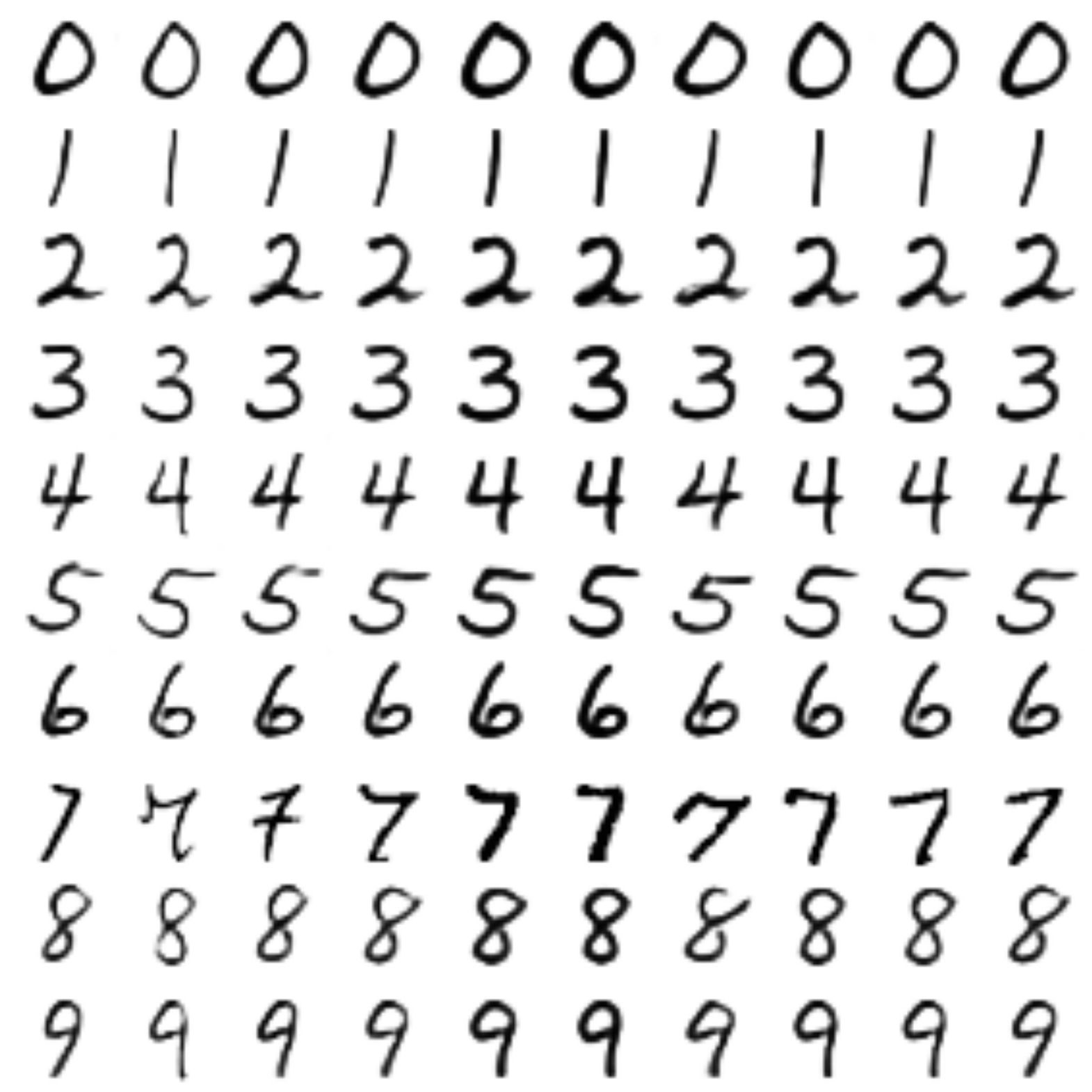
Generated digits of each label sampled from N (0 | I)

Learning process

Gifs

Style transfer

“7” was taken as a basis, from the style of which the remaining figures were already created (here $\ dim Z = 8$ ).

So it was with a simple CVAE :

And so it became:

Conclusion

In my opinion, it turned out very well. Having gone from the simplest auto-encoders , we got to generative models, namely to VAE , GAN , understood what conditional models are, and why metric is important.
We also learned to use keras and combine it with bare tensorflow .

Thank you all for your attention, I hope it was interesting!

Repository with all laptops

Useful links and literature

Original article:
[1] Autoencoding beyond pixels using a learned similarity metric, Larsen et al, 2016, https://arxiv.org/abs/1512.09300

Tutorial on VAE :
[2] Tutorial on Variational Autoencoders, Carl Doersch , 2016, https : //arxiv.org/abs/1606.05908

Tutorial on using keras with tensorflow :
[3] https://blog.keras.io/keras-as-a-simplified-interface-to-tensorflow-tutorial.html

Tags:

Auto Encoders in Keras Part 6: VAE + GAN

Content

We will examine in more detail why the restored images are blurry.

Connecting VAE and GAN

Code

results

Comparison with simple CVAE

Learning process

Style transfer

Conclusion

Useful links and literature

Also popular now: