December 2, 2016 at 21:33
Vacation schedule template (or training schedule or other schedule) in MS Excel file
I work as a small leader and have the responsibility of compiling and keeping up to date the vacation schedule of my department. This schedule is compiled at the end of the year for the next year and is provided to the personnel department of the organization. At the same time, the personnel department requires providing it in the format of a table-list, but I myself need a graphic format for work. In addition, due to the constant transfer of employee vacations, this schedule must be kept up to date.
Do not do unnecessary work and all that can be automated for me is a life principle. In this article I want to share the experience of creating MS EXCEL graph file. Perhaps the resulting template or this experience will be useful to you.
For those who need this template and who do not want to bother with how it works - right awayLink for viewing and downloading .
For those interested in the construction, the following description.
So. The format required by HR officers is depicted in the picture below (all surnames and positions are fictitious):
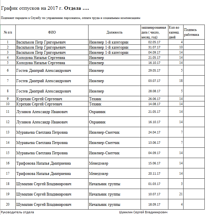
Features of this format:
1. Separate lines of vacation are included in the table in separate lines
2. The dates of the vacation start and duration are indicated in the table
3. The list is sorted alphabetically by the names of employees and by increasing start dates
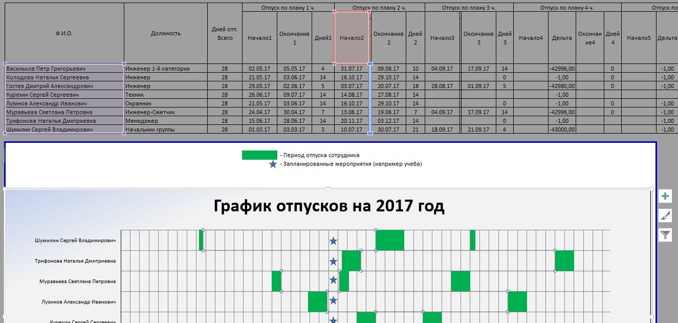
I also need a vacation schedule for my employees, but I would like to have it in the form of a clear calendar schedule (diagram), where the vacation periods of employees are reflected along the time axis. And in the end I made it - like this:
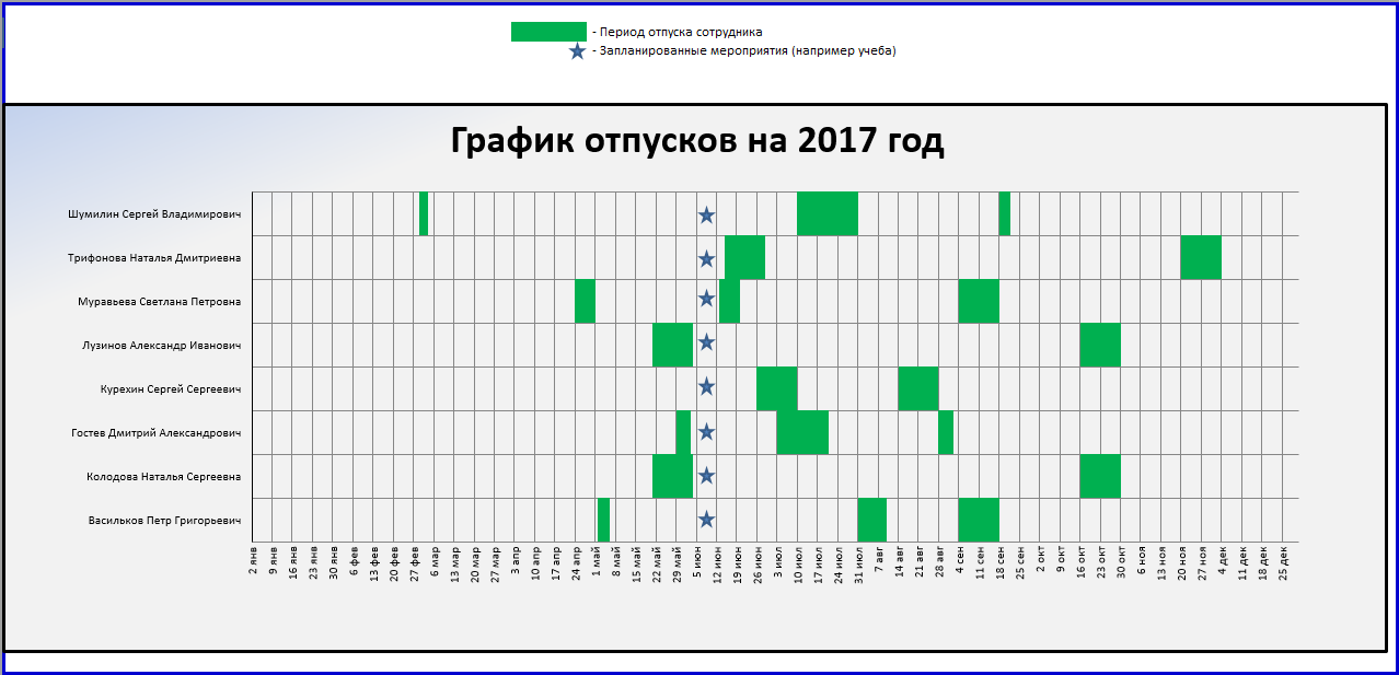
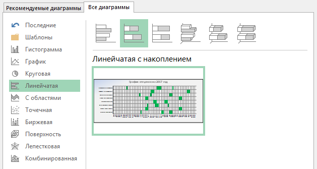
To create a graph of this form, I used the built-in diagram designer in MS EXCEL and the type of bar “Linear with accumulation”.
In order for the horizontal axis of the chart to look like a timeline, the following settings are needed:
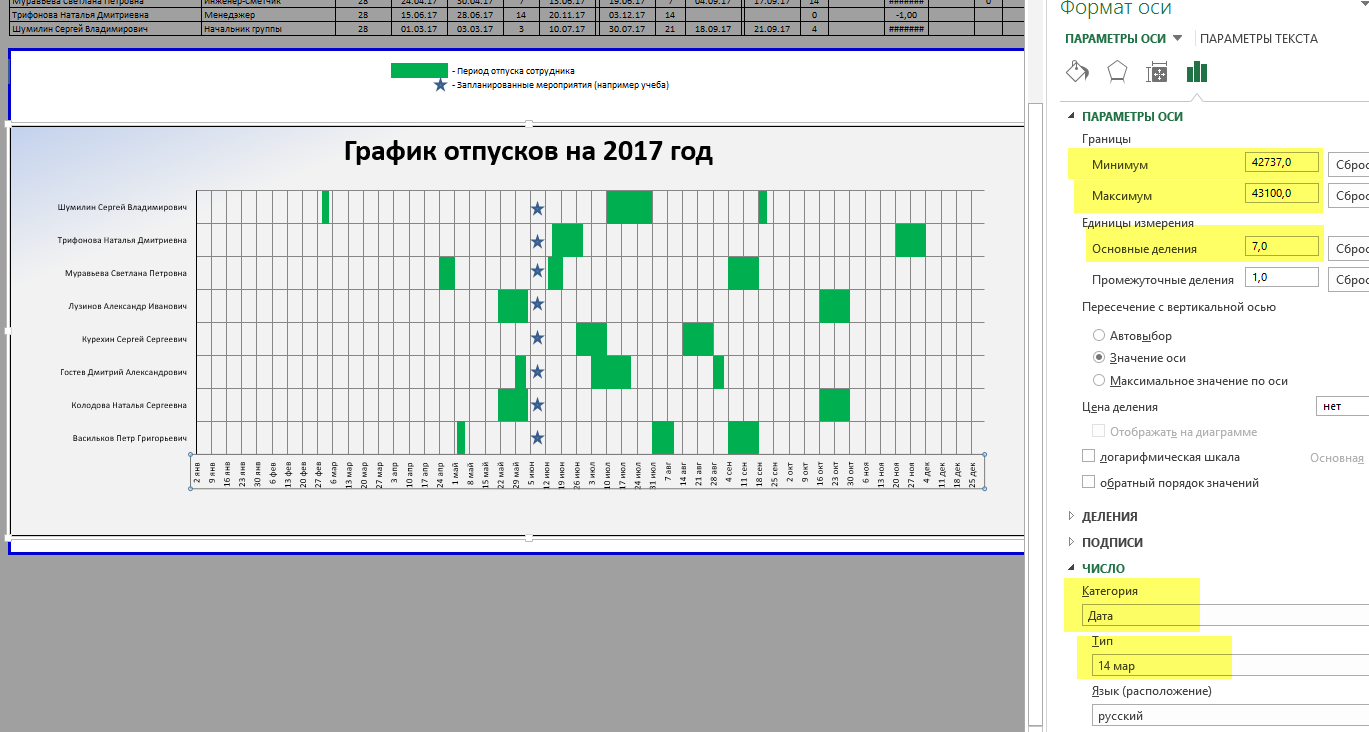
The maximum and minimum correspond to the numerical values of the dates of the beginning and end of the year. So that the seven-day grid coincides with the real weeks for the start date of the year, it is better not to take 01.01, but Monday closest to this date.
As a starting point for this chart formation, a table located above the chart is used. The printable area of the page is set so that it does not appear.
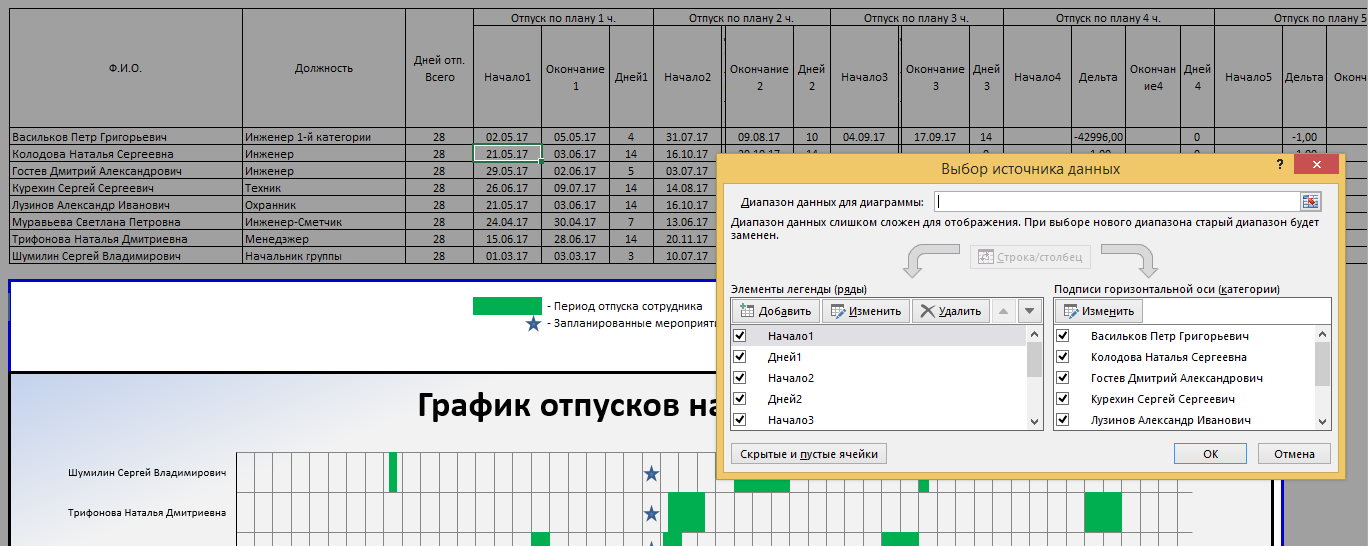
In fact, the chart reflects not only the periods of holidays, but also gaps between them (the settings display the holidays with green fill color, and breaks - without fill, that is, transparent).
This is the transparent period from the start of time to the start date of the first vacation of the year. The value in the "Start1" column is used.
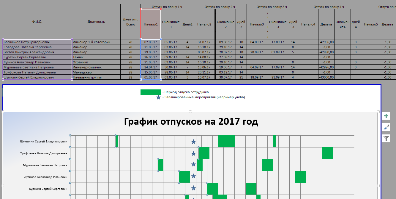
This is the first vacation displayed in green. The value in the “Days 1” column is used - the duration of the first vacation period:
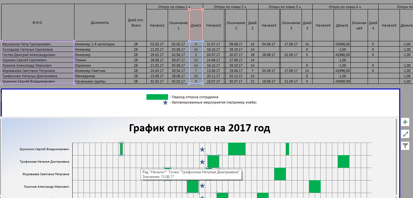
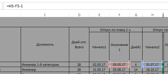
My "Days 1" column is calculated by the formula:
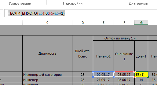
Plus one day because the end date of the vacation is its last day, and not the first working day.
This is the transparent period from the end of the first vacation to the beginning of the second.
It is also considered a formula, and since this value does not have user value - the column in the table is as narrow as possible.
Here I just want to say “well and so on ...”, in general, green vacation periods are constructed similarly to row 2, and transparent intervals between them are similar to row 3. For my task, 5 periods were enough - this is the current template limitation, which can be overcome by continuing the width of the table (how much patience you have).
They just need a list !?
Not to keep the same data in 2 places, not to create the possibility of their divergence - for me a matter of honor. Although it was necessary to spend time, it’s better to enter the formulas once than edit the data each time. There are no difficulties here - just links from a sheet containing a form for personnel officers to cells all in the same source table.
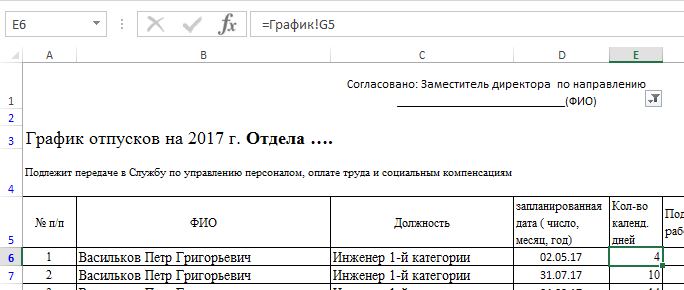
These links are filled in each row of the cell from B to E. For each row from the source table (each employee), respectively, the number of possible vacation periods is created - 5 rows in this table. For example, field E “Number of calendars. days ”, for the first employee completed:
For the next employee, the links will be to the same columns and to the next row (it was rather difficult to fill out because the form was transposed, but I did not understand how to copy the formulas with transposition).
Notice that column E has a filter. It is needed in order to display only filled vacation periods (configured not to display 0).
It remains to automate row numbering (first column). In the first line, I put the number “1” in my hands, for the rest I use the formula “= A6 + IF (E7 = 0; 0; 1)” (using the example of the 2nd line).
That's all. Thank you for attention
Do not do unnecessary work and all that can be automated for me is a life principle. In this article I want to share the experience of creating MS EXCEL graph file. Perhaps the resulting template or this experience will be useful to you.
For those who need this template and who do not want to bother with how it works - right awayLink for viewing and downloading .
For those interested in the construction, the following description.
The occurrence of the task
So. The format required by HR officers is depicted in the picture below (all surnames and positions are fictitious):
Features of this format:
1. Separate lines of vacation are included in the table in separate lines
2. The dates of the vacation start and duration are indicated in the table
3. The list is sorted alphabetically by the names of employees and by increasing start dates
Graph is a graph.
I also need a vacation schedule for my employees, but I would like to have it in the form of a clear calendar schedule (diagram), where the vacation periods of employees are reflected along the time axis. And in the end I made it - like this:
How is this done
To create a graph of this form, I used the built-in diagram designer in MS EXCEL and the type of bar “Linear with accumulation”.
In order for the horizontal axis of the chart to look like a timeline, the following settings are needed:
The maximum and minimum correspond to the numerical values of the dates of the beginning and end of the year. So that the seven-day grid coincides with the real weeks for the start date of the year, it is better not to take 01.01, but Monday closest to this date.
As a starting point for this chart formation, a table located above the chart is used. The printable area of the page is set so that it does not appear.
In fact, the chart reflects not only the periods of holidays, but also gaps between them (the settings display the holidays with green fill color, and breaks - without fill, that is, transparent).
First row
This is the transparent period from the start of time to the start date of the first vacation of the year. The value in the "Start1" column is used.
Second row
This is the first vacation displayed in green. The value in the “Days 1” column is used - the duration of the first vacation period:
My "Days 1" column is calculated by the formula:
Plus one day because the end date of the vacation is its last day, and not the first working day.
Third row
This is the transparent period from the end of the first vacation to the beginning of the second.
It is also considered a formula, and since this value does not have user value - the column in the table is as narrow as possible.
Subsequent rows
Here I just want to say “well and so on ...”, in general, green vacation periods are constructed similarly to row 2, and transparent intervals between them are similar to row 3. For my task, 5 periods were enough - this is the current template limitation, which can be overcome by continuing the width of the table (how much patience you have).
And what about the personnel officers?
They just need a list !?
Not to keep the same data in 2 places, not to create the possibility of their divergence - for me a matter of honor. Although it was necessary to spend time, it’s better to enter the formulas once than edit the data each time. There are no difficulties here - just links from a sheet containing a form for personnel officers to cells all in the same source table.
These links are filled in each row of the cell from B to E. For each row from the source table (each employee), respectively, the number of possible vacation periods is created - 5 rows in this table. For example, field E “Number of calendars. days ”, for the first employee completed:
1st line - "= Schedule! G5"
2nd line - "= Schedule! K5"
3rd line - "= Schedule! O5"
4th line - "= Schedule! S5"
5th line - " = Graph! W5 "
For the next employee, the links will be to the same columns and to the next row (it was rather difficult to fill out because the form was transposed, but I did not understand how to copy the formulas with transposition).
Notice that column E has a filter. It is needed in order to display only filled vacation periods (configured not to display 0).
It remains to automate row numbering (first column). In the first line, I put the number “1” in my hands, for the rest I use the formula “= A6 + IF (E7 = 0; 0; 1)” (using the example of the 2nd line).
That's all. Thank you for attention