Automation of measurement of the harmonic coefficient of a generator using a digital oscilloscope and MATLAB
In practice, sometimes the problem arises of measuring the harmonic coefficient (Kg) of a signal generator. Such a generator can be either analog or digital. For example, a generator on an operational amplifier, an integrated timer (NE555), a microcontroller (MK) or a programmable logic integrated circuit (FPGA), or a digital signal processor (DSP), with an output in the form of pulse-width modulation (PWM) or a digital-to-analog signal converter (DAC). If it is necessary to generate a harmonic signal, a low-pass filter (LPF) is installed at the output of the PWM or DAC, which smooths the step-like waveform and reduces Kg. In the general case, the measurement of Kg allows you to control the operation of both software algorithms and hardware nodes.
Kg can be measured using various instruments, for example, in the article“Measurement of the harmonic coefficient of the voltage signal specified in the time domain” provides several options for measuring this parameter, both traditional measuring instruments and promising ones. But I want to note that these devices are more specialized than, for example, a digital oscilloscope or multimeter. Therefore, not every engineer or radio amateur dares to buy such a device.
In order to understand how to measure Kg using improvised tools, you should look at its formula. For example, in the article “The coefficient of nonlinear distortion”The physical meaning of this parameter is described in detail. A simple formula that uses only the harmonics of the signal. Thus, if we measure the amplitudes of the harmonics of the signal at the output of the generator, then the solution to the problem of measuring Kr will be reduced to one formula.
Digital oscilloscopes may include the Fast Fourier Transform (FFT) option. In this case, the oscilloscope switches to the FFT measurement mode, and then with the help of markers, the harmonic amplitudes are measured and recorded on a piece of paper.
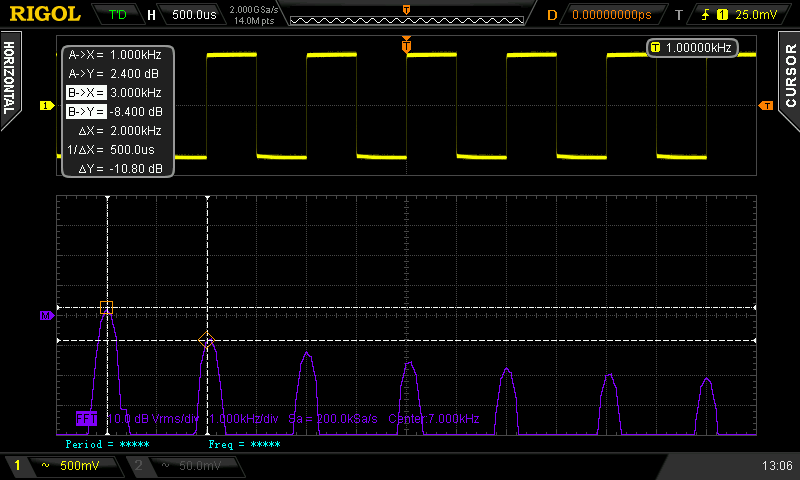
This usually happens, but firstly, it takes a long time, because measurements are made manually. And secondly, the duration of the signal sampling, and therefore the resolution of the FFT in frequency, as a rule, is significantly limited. Another thing is if using an oscilloscope to capture a sample of the signal of the desired length, for the subsequent calculation of the spectrum is already on the computer.
Most digital oscilloscopes with a remote interface, such as USB or Ethernet, can handle capturing a temporary sample of a signal and transferring it to a computer. And for calculating Kg from the spectrum, you can choose Matlab. Moreover, in the presence of the Instrument Control Toolbox, remote capture of the signal is made directly from Matlab.
But before using the method of calculating Kg from the spectrum, one would need to make sure that the oscilloscope is suitable. According to the study, which can be found in the article “Analytic Method for the Computation of the Total Harmonic Distortion by the Cauchy Method of Residues” , the Kg meander, as well as the signals received after filtering the meander with filters of various orders, have certain values, which in this case may be benchmarks. To check, you will need a rectangular pulse generator, which must be connected to an oscilloscope.

As well as relevant filters that can be implemented programmatically using the Signal Processing Toolbox.

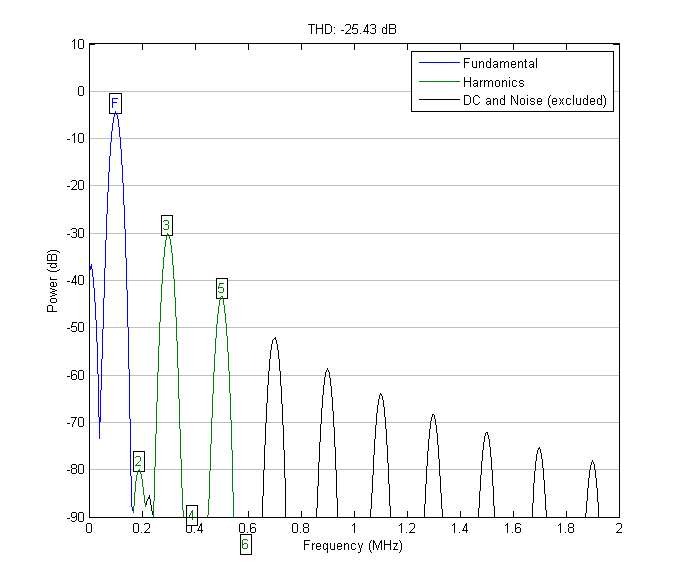
The spectrum of the output signal of the rectangular pulse generator. Kg = 43.98%
The spectrum at the output of a Butterworth filter of the second order. Kg = 5.36%
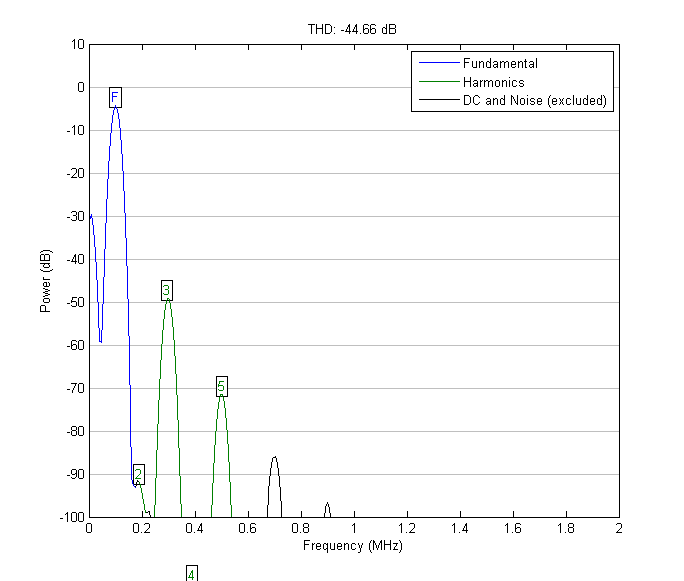
The spectrum at the fourth-order Butterworth filter output. Kg = 0.59%
A small explanation for the graphs: the logarithmic values of THD in the caps correspond only to the first 5 harmonics, therefore these values differ from the analogous ones, for which a larger number of harmonics is provided.
It should be noted that Kg at the output of the filters completely coincide with the calculated ones. But Kg for a rectangular signal is less than calculated, because the rectangular waveform spectrum damps slowly, and several tens of harmonics may be needed to achieve the calculated value - there's nothing to be done.
To automate the measurement of Kg, in addition to the previous script, you may need to support the commands of the tested generator using the Instrument Control Toolbox, but this is only if the device has a remote interface. For example, if commands are implemented as a Command-line Interface (CLI), then everything should be simple.
Actually, in this way Kg of the generator, which was developed on the basis of FPGA, was measured in a module designed to test analog transmission systems. As an example, below are the graphs of the spectra and the values of Kg directly at the output of the DAC (ADC in the figure) and after the filter link of type k, as well as the necessary script for plotting.
The signal and its spectrum at the output of the DAC, Kg = 28.3%
The signal and its spectrum at the output of a filter unit of type k, Kr = 2.5%
It should be noted that all this work was carried out only to assess the worst value Kr of the maximum frequency of the generator. In the working frequency band from 200 Hz to 62 kHz, Kg did not exceed 0.34%. For these frequencies, the graphs of the signals and spectra are no longer so interesting.
Thus, using the example of a generator built on an FPGA with a connected DAC and additional signal filtering using a low-pass filter type k, it is shown that the measurement of Kg at various points in the circuit can be carried out using a digital oscilloscope connected to a computer and Matlab. Such a mechanism can significantly reduce the time to evaluate the quality of the device’s functioning and saves the engineer from the routine of computing.
Kg can be measured using various instruments, for example, in the article“Measurement of the harmonic coefficient of the voltage signal specified in the time domain” provides several options for measuring this parameter, both traditional measuring instruments and promising ones. But I want to note that these devices are more specialized than, for example, a digital oscilloscope or multimeter. Therefore, not every engineer or radio amateur dares to buy such a device.
In order to understand how to measure Kg using improvised tools, you should look at its formula. For example, in the article “The coefficient of nonlinear distortion”The physical meaning of this parameter is described in detail. A simple formula that uses only the harmonics of the signal. Thus, if we measure the amplitudes of the harmonics of the signal at the output of the generator, then the solution to the problem of measuring Kr will be reduced to one formula.
Digital oscilloscopes may include the Fast Fourier Transform (FFT) option. In this case, the oscilloscope switches to the FFT measurement mode, and then with the help of markers, the harmonic amplitudes are measured and recorded on a piece of paper.
This usually happens, but firstly, it takes a long time, because measurements are made manually. And secondly, the duration of the signal sampling, and therefore the resolution of the FFT in frequency, as a rule, is significantly limited. Another thing is if using an oscilloscope to capture a sample of the signal of the desired length, for the subsequent calculation of the spectrum is already on the computer.
Most digital oscilloscopes with a remote interface, such as USB or Ethernet, can handle capturing a temporary sample of a signal and transferring it to a computer. And for calculating Kg from the spectrum, you can choose Matlab. Moreover, in the presence of the Instrument Control Toolbox, remote capture of the signal is made directly from Matlab.
function [osc_data,fs] = osc_capture_ds2202()
ds2000 = visa('ni','USB0::0x1AB1::0x04B0::DS2A142900939::INSTR');   % Create VISA object.
ds2000.InputBufferSize = 2e6;
fopen(ds2000);
fprintf(ds2000,':CHAN1:BWLimit 20M');   % Set BandWidth Limit to 20MHz.
fprintf(ds2000,':ACQ:MDEPth 140000');   % Set Memory Depth from several typical values.
fs = str2double(query(ds2000,':ACQ:SRATe?')); % Get Sample Rate.
%% Setup Waveform
fprintf(ds2000,':STOP');    % Stop oscilloscope.
fprintf(ds2000,':WAV:SOURce CHAN1');
fprintf(ds2000,':WAV:MODE RAW');
fprintf(ds2000,':WAVeform:FORMat ASCII');
fprintf(ds2000,':WAV:POINts 131072');   % Number of points that must be less than MDEPth.
fprintf(ds2000,':WAV:RESet');
fprintf(ds2000,':WAV:BEGin');
pause(5);   % Wait the end of the acquisition.
%% Get Waveform
while true
    status = query(ds2000,':WAV:STATus?');
    pause(1);   % Not neccesary, but...
    [state,rem] = strtok(status,',');
    len = strtok(sscanf(rem,'%s'),',');
    if eq(len,'0')
        break;
    end
    if eq(state(1),'I')
        osc_data = cell2mat(textscan(query(ds2000,':WAV:DATA?'),'%f','delimiter',','));
        break;
    else
        osc_data = cell2mat(textscan(query(ds2000,':WAV:DATA?'),'%f','delimiter',','));
    end
end
fprintf(ds2000,':WAV:END');
fprintf(ds2000,':RUN'); % Run the oscilloscope.
%% Delete instrument object
fclose(ds2000);
delete(ds2000);
clear ds2000;
But before using the method of calculating Kg from the spectrum, one would need to make sure that the oscilloscope is suitable. According to the study, which can be found in the article “Analytic Method for the Computation of the Total Harmonic Distortion by the Cauchy Method of Residues” , the Kg meander, as well as the signals received after filtering the meander with filters of various orders, have certain values, which in this case may be benchmarks. To check, you will need a rectangular pulse generator, which must be connected to an oscilloscope.
As well as relevant filters that can be implemented programmatically using the Signal Processing Toolbox.
clear all
clc
%% Signal Acquisition
[s,fs] = osc_capture_ds2202();  % s - signal, fs - sample frequency.
%% Setup parameters
number_of_harmonics = 11; % Number of harmonics (including the fundamenal)...
    % to use in the THD calculation.
L = length(s);  % Length of the signal for FFT computing. It is used only for plot.
T = 1/fs;
t = (0:L-1)*T;
s_ac = s-mean(s); % Remove DC level. It is not neccesary for thd function.
s_ac = s_ac/max(abs(s_ac)); % Normalize signal. As above for thd.
%% Estimate the THD of the signal
[thd_dBc,harmpow,harmfreq] = thd(s_ac,fs,number_of_harmonics);
thd_perc = 10^(thd_dBc/20)*100  % Convert dB to Percents and display result.
figure(2);
thd(s_ac,fs);   % Plot the Spectrum of the signal.
%% Apply Butterworth filter to signal and estimate THD for filtered signal
[lpFilter_b_II, lpFilter_a_II] = butter(2,2*harmfreq(1)/fs,'low');  % Design B-II filter.
filtII_s_ac = filter(lpFilter_b_II, lpFilter_a_II, s_ac);   % Apply B-II filter to signal.
thd_perc_BII = 10^(thd(filtII_s_ac,fs,number_of_harmonics)/20)*100  % Convert dB to Percents and display result.
figure(3);
thd(filtII_s_ac,fs);   % Plot the Spectrum of the B-II filter.
[lpFilter_b_IV, lpFilter_a_IV] = butter(4,2*harmfreq(1)/fs,'low');  % Design B-IV filter.
filtIV_s_ac = filter(lpFilter_b_IV, lpFilter_a_IV, s_ac);   % Apply B-IV filter to signal.
thd_perc_BIV = 10^(thd(filtIV_s_ac,fs,number_of_harmonics)/20)*100  % Convert dB to Percents and display result.
figure(4);
thd(filtIV_s_ac,fs);   % Plot the Spectrum of the B-IV filter.
The spectrum of the output signal of the rectangular pulse generator. Kg = 43.98%
The spectrum at the output of a Butterworth filter of the second order. Kg = 5.36%
The spectrum at the fourth-order Butterworth filter output. Kg = 0.59%
A small explanation for the graphs: the logarithmic values of THD in the caps correspond only to the first 5 harmonics, therefore these values differ from the analogous ones, for which a larger number of harmonics is provided.
It should be noted that Kg at the output of the filters completely coincide with the calculated ones. But Kg for a rectangular signal is less than calculated, because the rectangular waveform spectrum damps slowly, and several tens of harmonics may be needed to achieve the calculated value - there's nothing to be done.
To automate the measurement of Kg, in addition to the previous script, you may need to support the commands of the tested generator using the Instrument Control Toolbox, but this is only if the device has a remote interface. For example, if commands are implemented as a Command-line Interface (CLI), then everything should be simple.
[qty,b5_comport_list,~,b5] = b5_open_test; % Search connected devices.
if qty
b5.Port = b5_comport_list{1}; % Assign port to first device.
fopen(b5);
disp(b5_command(b5,'versions',.1)); % Display Versions of MCU and FPGA.
disp(b5_command(b5,'sn',.1)); % Display Serial Number.
b5_command(b5,'outrfreq 101050',.1); % Set output frequency.
b5_command(b5,'outrlvl 0',.1); % Set output level.
b5_command(b5,'outimp 600',.1); % Set output impedance.
b5_command(b5,'outpath output',.1); % Connect generator to output connector.
fclose(b5); % Close port.
delete(b5); % Clear buffer.
clear b5 % Remove var from memory.
else
disp('b5-vf is not connected');
delete(b5); % Clear buffer.
clear b5 % Remove var from memory.
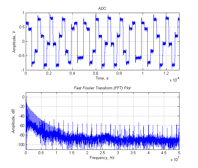
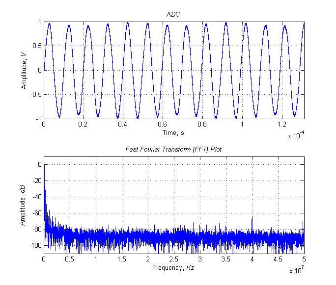
endActually, in this way Kg of the generator, which was developed on the basis of FPGA, was measured in a module designed to test analog transmission systems. As an example, below are the graphs of the spectra and the values of Kg directly at the output of the DAC (ADC in the figure) and after the filter link of type k, as well as the necessary script for plotting.
%% Window
win = tukeywin(length(s_ac),1); % Generate window.
% win = 1; % Disable window.
s_ac_win = s_ac.*win;   % Apply the window.
%% FFT
nfft = 2^nextpow2(L);   %% FFT length
fft_s_ac_win = fft(s_ac_win,nfft)/L;
f = fs/2*linspace(0,1,nfft/2+1);
win_scale = 1/mean(win);    %% Normalization the result
fft_s_ac_win_lin = 2*win_scale*abs(fft_s_ac_win(1:nfft/2+1));
fft_s_ac_win_log = 20*log10(fft_s_ac_win_lin);
%% Fig 1
figure(1);
subplot(2,1,1), plot(t,s_ac), axis([0 max(t) -max(abs(s_ac)) max(abs(s_ac))]), grid on;
title('\itADC','fontsize',10);
xlabel('Time, \its','fontsize',10), ylabel('Amplitude, \itV','fontsize',10);
subplot(2,1,2), plot(f,fft_s_ac_win_log), axis([0 fs/2 -110 10]), grid on;
title('\itFast Fourier Transform (FFT) Plot','fontsize',10);
xlabel('Frequency, \itHz','fontsize',10), ylabel('Amplitude, \itdB','fontsize',10);
The signal and its spectrum at the output of the DAC, Kg = 28.3%
The signal and its spectrum at the output of a filter unit of type k, Kr = 2.5%
It should be noted that all this work was carried out only to assess the worst value Kr of the maximum frequency of the generator. In the working frequency band from 200 Hz to 62 kHz, Kg did not exceed 0.34%. For these frequencies, the graphs of the signals and spectra are no longer so interesting.
Thus, using the example of a generator built on an FPGA with a connected DAC and additional signal filtering using a low-pass filter type k, it is shown that the measurement of Kg at various points in the circuit can be carried out using a digital oscilloscope connected to a computer and Matlab. Such a mechanism can significantly reduce the time to evaluate the quality of the device’s functioning and saves the engineer from the routine of computing.