We solve the "First open contest" from Mail.ru on Data Science using Azure ML (introduction to Azure ML)
Now the ML Boot Camp competition is taking place , in which it is necessary to predict the time for which 2 matrices of sizes mxk and kxn will be multiplied on this computer system, if it is known how much this problem was solved on other computer systems with different matrix sizes ( exact rules ). Let's try to solve this problem of regression not using standard tools and libraries (R, Python and panda), but using a cloud product from Microsoft: Azure ML . For our purposes, free access is suitable, for which even a trial Azure account is enough. Everyone who wants to get a quick guide on setting up and using Azure ML in general and ML Studio in particular, using the example of solving real-life tasks, are invited to cat.

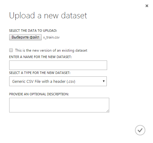
We’ll open ML Studio: we will create one new experiment (in terms of Azure ML it represents a complete solution to the problem - from reading the input data to receiving the answer, then it can be converted to Web Service) and two new data sources (dataset) to represent the input data (one for a set of characteristics, another for values). Download the training sample files (x_train.csv and y_train.csv) from the ML Boot Camp csv website. To add a data source, you need to select the "Dataset" item in the menu on the left and click "New" in the lower left corner, the following window will appear:
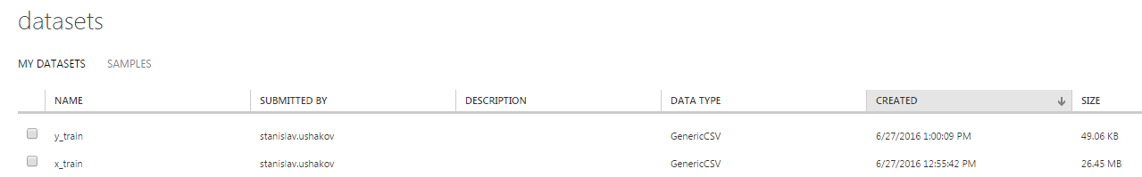
Specify the path to the x_train.csv file, give this data source the name x_train. Also create a y_train data source. Now both of these data sources are shown on the Datasets tab:
It's time to create an experiment, for this in the menu on the left, select the item “Experiments”, click “New” in the lower left and select “Blank Experiment”. In the line at the top you can give it a suitable name, as a result, we get the following scope for our Data Science operations:

As you can see, on the left is a menu that lists all the possible operations that can be added to the experiment, such as: input and output of data, selection of columns, various methods of regression, classification, etc. All of them will be added to our experiment by simply dragging and dropping different operations between themselves.
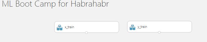
Now we need to show what we want to use as input for the task. In the menu on the left, select the topmost item “Saved Datasets”, then “My Datasets”, in the list we select the data sources “x_train” and “y_train” that we created and drag them to the workspace of the experiment, as a result we get:
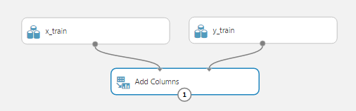
Now we need to combine the columns of these two data sources, because all Azure ML methods work with one table (data frame), in which we need to specify the column that is the training value. To do this, use the Add Columns module. Hint: a search on the modules will help you find the module by keywords or make sure that such a module does not yet exist. Drag the operation "Add Columns" into the workspace and connect its two upper points for data entry with our data sources x_train and y_train, respectively. This operation has no parameters, so you do not need to configure anything additionally. We get:
To see how our data now looks. Run the experiment by clicking the "Run" button on the bottom line. After the experiment is successfully completed, you can click on the output of the “Add Columns” operation and select the “Visualize” action:


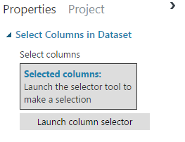
The properties window allows you to see the columns, the first rows, for each characteristic: average, median, histogram, etc. We see that in our table there are 952 columns (signs), and from them we must choose significant ones, those that will help us in solving our problem. The selection of features is one of the most complex and non-deterministic operations in Data Science, so now for simplicity we will choose several features that are significant at first glance. The module that will help us do this is called Select Columns in Dataset. Add it to the workspace, connect it to the Add Columns operation. Now, in the “Select Columns in Dataset” parameters, we indicate what signs we want to leave. To do this, select the “Select Columns in Dataset” module, in the properties in the right pane, click “Launch column selector”:
Now add the names of the columns that we want to leave (this is not the optimal choice of columns), do not forget to add the “time” column:

Run the experiment again, make sure that only the columns that are selected remain in the resulting table. Now the last step in preparing the data: we will divide the data into training and test samples in the proportion of 70:30. To do this, find and place the “Split Data” module in the workspace, set “Fraction of rows in the first output dataset” to 0.7 in its settings. We get:

Now we are ready to finally use some kind of regression method. The methods are listed in the menu on the left: “Machine Learning”, “Initialize Model”, “Regression”:

First, let's try the decision tree forest method: “Decision Forest Regression”. Add it to the workspace, as well as the “Train model” module. This module has two inputs: one is connected to the algorithm (in our case, “Decision Forest Regression”), the other to the data from the training sample (left output of the “Split Data” module). The experiment now looks like this:

The red circle in the “Train model” module tells us that it has the required parameters that we have not tuned up: it needs to indicate which sign we are trying to predict (in our case, this is time). Click “Launch column selector”, add a single time column. Note that the method itself has default settings that allow it to start without manual reconfiguration. Of course, to get good results, you need to try various combinations of parameters that will be specific to each method. Now the experiment can be started, the forest of trees will be built, they can even be viewed by calling up the already familiar “Visualize” window. After training the model, it would be good to test it on a test (validation) sample, which represents 30% of the initial data. To do this, use the “Score Model” module, combining its first input with the output of the Train model module (trained model), and the second with the second output of the Split Data module. Now the sequence of operations looks like this:

You can run the experiment again and see the output of the “Score model”:

2 new columns were added: “Scored Label Mean” (mean of the predicted value) and “Scored Label Standard Deviation” (standard deviation of the predicted value from the actual). You can also build a scatter plot (scatter plot) for the predicted and actual values (visible in the figure). Now we find out its accuracy using the Evaluate Model module, which is connected to the Score Model module.

The output of the Evaluate Model module contains information about the accuracy of the method on our test data, including absolute and relative errors:

Of course, the method is not ideal, but we did not configure it at all.
Let's try another method based on decision trees: “Boosted Decision Tree Regression”. In the same way as for the first method, add the “Train Model” and “Score Model” modules, start the experiment, see the output of the “Score Model” module for the new method. Note that only one column was added that represents the predicted value: “Scored Labels”, you can also build a scatter chart for it:

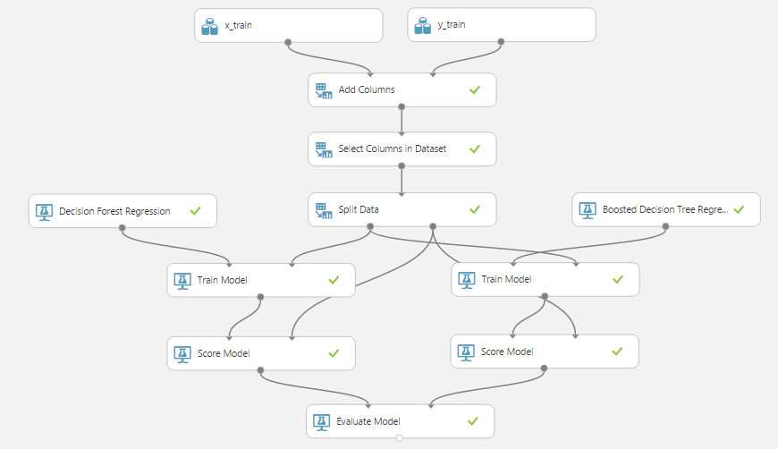
Now we compare the accuracy of these two methods using the already added “Evaluate Model” module, for this we connect its right input with the output "Score Model" of the second method. As a result, we obtain the following sequence of operations:
Let's look at the output of the Evaluate Model module:

Now we can compare the methods with each other and choose the one whose accuracy (in the sense necessary for our task) is higher.
We have trained methods, we know their accuracy - it's time to test them in battle. Download the x_test.csv file, which contains the data for which we must predict the time of matrix multiplication. To use the trained method, we need:
As a result, we get the following experiment:

You can download the obtained csv file by clicking on the output of the “Convert to CSV” module and selecting the “Download” item. Now we will delete the first line (with the name) from the resulting csv, upload it to the ML Boot Camp website. Works! But accuracy is poor.
Consider a few modules that will help improve the accuracy of regression.
I like Azure ML, it allows you to quickly prototype a solution to a problem, and then delve into customizing and optimizing its solution.
The experiment is posted in the gallery and is open to all comers at: gallery.cortanaintelligence.com/Experiment/ML-Boot-Camp-from-Mail-ru-1
Take part in the contest! Anyone who can get a MAPE error of less than 0.1, write, the author will be pleased.
Creating data sources
We’ll open ML Studio: we will create one new experiment (in terms of Azure ML it represents a complete solution to the problem - from reading the input data to receiving the answer, then it can be converted to Web Service) and two new data sources (dataset) to represent the input data (one for a set of characteristics, another for values). Download the training sample files (x_train.csv and y_train.csv) from the ML Boot Camp csv website. To add a data source, you need to select the "Dataset" item in the menu on the left and click "New" in the lower left corner, the following window will appear:
Specify the path to the x_train.csv file, give this data source the name x_train. Also create a y_train data source. Now both of these data sources are shown on the Datasets tab:
Create an experiment, select characteristics
It's time to create an experiment, for this in the menu on the left, select the item “Experiments”, click “New” in the lower left and select “Blank Experiment”. In the line at the top you can give it a suitable name, as a result, we get the following scope for our Data Science operations:
As you can see, on the left is a menu that lists all the possible operations that can be added to the experiment, such as: input and output of data, selection of columns, various methods of regression, classification, etc. All of them will be added to our experiment by simply dragging and dropping different operations between themselves.
Now we need to show what we want to use as input for the task. In the menu on the left, select the topmost item “Saved Datasets”, then “My Datasets”, in the list we select the data sources “x_train” and “y_train” that we created and drag them to the workspace of the experiment, as a result we get:
Now we need to combine the columns of these two data sources, because all Azure ML methods work with one table (data frame), in which we need to specify the column that is the training value. To do this, use the Add Columns module. Hint: a search on the modules will help you find the module by keywords or make sure that such a module does not yet exist. Drag the operation "Add Columns" into the workspace and connect its two upper points for data entry with our data sources x_train and y_train, respectively. This operation has no parameters, so you do not need to configure anything additionally. We get:
To see how our data now looks. Run the experiment by clicking the "Run" button on the bottom line. After the experiment is successfully completed, you can click on the output of the “Add Columns” operation and select the “Visualize” action:
The properties window allows you to see the columns, the first rows, for each characteristic: average, median, histogram, etc. We see that in our table there are 952 columns (signs), and from them we must choose significant ones, those that will help us in solving our problem. The selection of features is one of the most complex and non-deterministic operations in Data Science, so now for simplicity we will choose several features that are significant at first glance. The module that will help us do this is called Select Columns in Dataset. Add it to the workspace, connect it to the Add Columns operation. Now, in the “Select Columns in Dataset” parameters, we indicate what signs we want to leave. To do this, select the “Select Columns in Dataset” module, in the properties in the right pane, click “Launch column selector”:
Now add the names of the columns that we want to leave (this is not the optimal choice of columns), do not forget to add the “time” column:
Run the experiment again, make sure that only the columns that are selected remain in the resulting table. Now the last step in preparing the data: we will divide the data into training and test samples in the proportion of 70:30. To do this, find and place the “Split Data” module in the workspace, set “Fraction of rows in the first output dataset” to 0.7 in its settings. We get:
Using Algorithms
Now we are ready to finally use some kind of regression method. The methods are listed in the menu on the left: “Machine Learning”, “Initialize Model”, “Regression”:
First, let's try the decision tree forest method: “Decision Forest Regression”. Add it to the workspace, as well as the “Train model” module. This module has two inputs: one is connected to the algorithm (in our case, “Decision Forest Regression”), the other to the data from the training sample (left output of the “Split Data” module). The experiment now looks like this:
The red circle in the “Train model” module tells us that it has the required parameters that we have not tuned up: it needs to indicate which sign we are trying to predict (in our case, this is time). Click “Launch column selector”, add a single time column. Note that the method itself has default settings that allow it to start without manual reconfiguration. Of course, to get good results, you need to try various combinations of parameters that will be specific to each method. Now the experiment can be started, the forest of trees will be built, they can even be viewed by calling up the already familiar “Visualize” window. After training the model, it would be good to test it on a test (validation) sample, which represents 30% of the initial data. To do this, use the “Score Model” module, combining its first input with the output of the Train model module (trained model), and the second with the second output of the Split Data module. Now the sequence of operations looks like this:
You can run the experiment again and see the output of the “Score model”:
2 new columns were added: “Scored Label Mean” (mean of the predicted value) and “Scored Label Standard Deviation” (standard deviation of the predicted value from the actual). You can also build a scatter plot (scatter plot) for the predicted and actual values (visible in the figure). Now we find out its accuracy using the Evaluate Model module, which is connected to the Score Model module.
The output of the Evaluate Model module contains information about the accuracy of the method on our test data, including absolute and relative errors:
Of course, the method is not ideal, but we did not configure it at all.
Adding a new method and comparing methods
Let's try another method based on decision trees: “Boosted Decision Tree Regression”. In the same way as for the first method, add the “Train Model” and “Score Model” modules, start the experiment, see the output of the “Score Model” module for the new method. Note that only one column was added that represents the predicted value: “Scored Labels”, you can also build a scatter chart for it:
Now we compare the accuracy of these two methods using the already added “Evaluate Model” module, for this we connect its right input with the output "Score Model" of the second method. As a result, we obtain the following sequence of operations:
Let's look at the output of the Evaluate Model module:
Now we can compare the methods with each other and choose the one whose accuracy (in the sense necessary for our task) is higher.
We solve the problem with real data
We have trained methods, we know their accuracy - it's time to test them in battle. Download the x_test.csv file, which contains the data for which we must predict the time of matrix multiplication. To use the trained method, we need:
- Add a new data source named x_test and data from the file x_test.csv.
- Drag the new x_test data source to the experiment workspace.
- Now we need to leave only those columns that participated in the training, copy the “Select Columns in Dataset” module, and remove the “time” column from the list of columns (since it is not in our test data).
- Now we can run our trained method on the prepared data, for this we add the “Score Model” operation, connect its first input to the output of the Train Model module of the Boosted Decision Tree Regression method, and the second input with the output of the just selected Select Columns in Dataset. "
- Now it remains only to bring the data to a format that can be downloaded as a solution to the ML Boot Camp website. To do this, add another “Select Columns in Dataset” module, in which we select only one column — our predicted “Scored Labels” values, and add the “Convert to CSV” module to its output.
As a result, we get the following experiment:
You can download the obtained csv file by clicking on the output of the “Convert to CSV” module and selecting the “Download” item. Now we will delete the first line (with the name) from the resulting csv, upload it to the ML Boot Camp website. Works! But accuracy is poor.
Further optimization
Consider a few modules that will help improve the accuracy of regression.
- Try different methods that can be found in the menu on the left.
- The “Filter Based Feature Selection” module will help you select features, which tries to select features that have the greatest predictive ability (using several different methods that are set in its properties). This module is added instead of the Select Columns in Dataset module.
- To assess which features are more useful in an already trained model, the Permutation Feature Importance module will help, which takes a trained model and a set of test data as input parameters.
- The “Tune Model Hyperparameters” module will help you select the method parameters, which will conduct a given number of method starts with various sets of parameters and show the accuracy of each run.
- As heavy artillery, you can use any R and Python scripts using the “Execute R Script” and “Execute Python Script” modules, respectively.
Conclusion
I like Azure ML, it allows you to quickly prototype a solution to a problem, and then delve into customizing and optimizing its solution.
The experiment is posted in the gallery and is open to all comers at: gallery.cortanaintelligence.com/Experiment/ML-Boot-Camp-from-Mail-ru-1
Take part in the contest! Anyone who can get a MAPE error of less than 0.1, write, the author will be pleased.