Forchun algorithm, implementation details
- Transfer
For the past few weeks, I've been working on implementing Forchun's algorithm in C ++. This algorithm takes a lot of 2D-points and builds a Voronoi diagram from them . If you do not know what a Voronoi diagram is, then take a look at the figure:
For each entry point, which is called a “site” (site), we need to find a set of points that are closer to this place than to all the others. Such sets of points form cells, which are shown in the image above.
It is noteworthy in the Fortune’s algorithm that it builds such diagrams over time. (which is optimal for the comparison algorithm), where - this is the number of places.
I am writing this article because I consider the implementation of this algorithm a very difficult task. At the moment it is the most difficult of the algorithms that I had to implement. Therefore, I want to share the problems that I encountered, and how to solve them.
As usual, the code is posted on github , and all the references I used are listed at the end of the article.
I will not explain how the algorithm works, because other people have already done it well. I can recommend to study these two articles: here and here . The second one is very curious - the author wrote an interactive Javascript demo, which is useful for understanding the operation of the algorithm. If you need a more formal approach with all the evidence, I recommend reading Chapter 7 of the book Computational Geometry, 3rd edition .
Moreover, I prefer to deal with implementation details that are not well documented. And they make the implementation of the algorithm so complicated. In particular, I will focus on the data structures used.
I just wrote the pseudo-code of the algorithm so that you get an idea of its global structure:
The first problem I encountered was the choice of how to store the Voronoi diagram.
I decided to use the data structure is widely used in computational geometry, which is called a doubly linked list of edges (doubly connected edge list, DCEL) .
My class
I will tell you in detail about each of them.
The class
The vertices of the cell are represented by a class
Here is the implementation of the semi-loggers
You may be wondering - what is half the floor? The edge in the Voronoi diagram is common to two adjacent cells. In the DCEL data structure, we divide these edges into two half-edges, one for each cell, and they are linked by a pointer
The figure below shows all these fields for the red half-rim:

Finally, the class
The standard way to implement an event queue is a priority queue. During the processing of the place and circle events, we may need to remove the circle events from the queue, because they are no longer valid. But most standard implementations of the priority queue do not allow deleting an element that is not on top. In particular, this also applies to
This problem can be solved in two ways. The first, simpler one is to add a flag to the events
The second method that I applied is not to use
The shoreline data structure is a complex part of the algorithm. In case of incorrect implementation there are no guarantees that the algorithm will be executed in. The key to obtaining such a time complexity is the use of a self-balancing tree. But it is easier said than done!
In most of the resources that I have studied (the two above-mentioned articles and the book of Computational Geometry ), it is advised to implement the coastline as a tree, in which the internal nodes indicate break points, and the leaves indicate arcs. But they say nothing about how to balance a tree. I think that such a model is not the best, and this is why:
Therefore, I decided to present the coastline differently. In my implementation, the coastline is also a tree, but all nodes represent arcs. This model does not have any of the listed disadvantages.
Here is the definition of the arc
The first three fields are used for tree structure. The field
To balance the coastline, I decided to use the red-black scheme . When writing code, I was inspired by the book Introduction to Algorithms . Chapter 13 describes two interesting algorithms,
However, I cannot use the method given in the book
The insert
The removal method taken from the book can be implemented without changes.
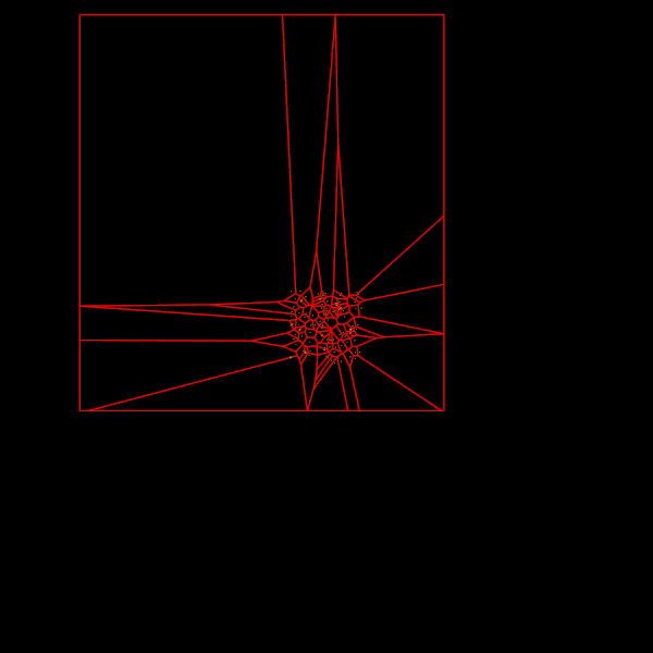
Here is the output of the Forchun algorithm described above:
There is a small problem with some edges of cells on the border of the image: they are not drawn because they are infinite.
Worse, the cell may not be a single fragment. For example, if we take three points on one line, then the middle point will have two infinite half-edges that are not connected together. This does not suit us very much, because we will not be able to access one of the semi-edges, because the cell is a linked list of edges.
To solve these problems, we will restrict the chart. By this I mean that we will limit each cell of the diagram so that they no longer have infinite edges and each cell is a closed polygon.
Fortunately, the Forchun algorithm allows us to quickly find infinite edges: they correspond to the semi-ridges that are still on the coastline by the end of the algorithm.
My restriction algorithm receives a rectangle (box) as input and consists of three steps:
Stage 1 is trivial - we just need to expand the rectangle if it does not contain a vertex.
Stage 2 is also quite simple - it consists of calculating the intersections between the rays and the rectangle.
Stage 3 is also not very complicated, only requires care. I do it in two stages. First, I add the points of the corners of the rectangle to the cells at the vertices of which they should be. Then I make it so that all the vertices of the cell are connected by semi-spans.
I recommend to study the code and ask questions if you need details about this part.
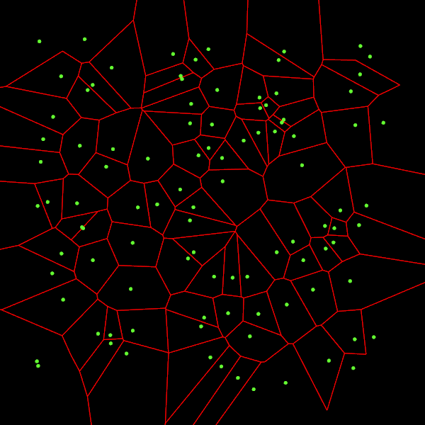
Here is the output diagram of the limiting algorithm:
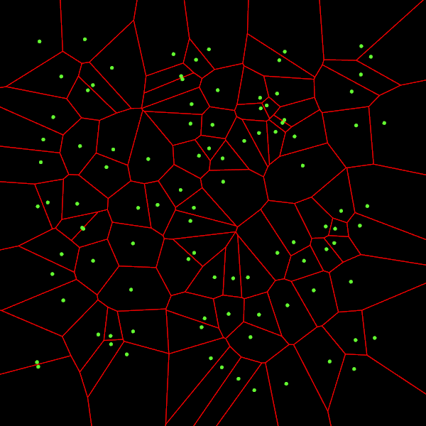
Now we see that all edges are drawn. And if you scale down, you can make sure that all cells are closed:
Fine! But the first image from the beginning of the article is better, right?
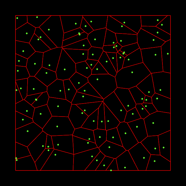
In many applications it is useful to have an intersection between the Voronoi diagram and the rectangle, as shown in the first image.
The good news is that after limiting the diagram, it is much easier to do this. The bad thing is that although the algorithm is not very complicated, we need to be careful.
The idea is as follows: we go around its semi-contour of each cell and check the intersection between the half-rim and the rectangle. Five cases are possible:
Yes, there are many cases. I created a picture to show them all:

The orange polygon is the source cell, and the red polygon is a truncated cell. Truncated semi-ribs are marked in red. Green edges are added to link the semi-ribs entering the rectangle with the semi-curbs facing the outside.
Applying this algorithm to the restricted diagram, we get the expected result:
The article was quite long. And I am sure that many aspects are still not clear to you. However, I hope it will be useful to you. Examine the code to get the details.
To summarize and make sure that we did not waste time in vain, I measured on my (cheap) laptop the time to calculate the Voronoi diagram for a different number of places:
I have nothing to compare these figures with, but it seems that it is incredibly fast!
For each entry point, which is called a “site” (site), we need to find a set of points that are closer to this place than to all the others. Such sets of points form cells, which are shown in the image above.
It is noteworthy in the Fortune’s algorithm that it builds such diagrams over time. (which is optimal for the comparison algorithm), where - this is the number of places.
I am writing this article because I consider the implementation of this algorithm a very difficult task. At the moment it is the most difficult of the algorithms that I had to implement. Therefore, I want to share the problems that I encountered, and how to solve them.
As usual, the code is posted on github , and all the references I used are listed at the end of the article.
Fortune's algorithm description
I will not explain how the algorithm works, because other people have already done it well. I can recommend to study these two articles: here and here . The second one is very curious - the author wrote an interactive Javascript demo, which is useful for understanding the operation of the algorithm. If you need a more formal approach with all the evidence, I recommend reading Chapter 7 of the book Computational Geometry, 3rd edition .
Moreover, I prefer to deal with implementation details that are not well documented. And they make the implementation of the algorithm so complicated. In particular, I will focus on the data structures used.
I just wrote the pseudo-code of the algorithm so that you get an idea of its global structure:
we add event of place to queue of events for each place
until the event queue is empty
    extract the top event
    if the event is a place event
        insert a new arc into the coastline
        check for new events of circles
    otherwise
        create a vertex in the diagram
        remove from the coastline constricted arc
        delete invalid events
        check for new events of circles
Chart data structure
The first problem I encountered was the choice of how to store the Voronoi diagram.
I decided to use the data structure is widely used in computational geometry, which is called a doubly linked list of edges (doubly connected edge list, DCEL) .
My class
VoronoiDiagramuses four containers as fields:classVoronoiDiagram
{public:
// ...private:
std::vector<Site> mSites;
std::vector<Face> mFaces;
std::list<Vertex> mVertices;
std::list<HalfEdge> mHalfEdges;
}I will tell you in detail about each of them.
The class
Sitedescribes the entry point. Each place has an index, which is useful for placing it in the queue, coordinates and a pointer to the cell ( face):structSite
{std::size_t index;
Vector2 point;
Face* face;
};The vertices of the cell are represented by a class
Vertex, they have only a coordinate field:structVertex
{
Vector2 point;
};Here is the implementation of the semi-loggers
structHalfEdge
{
    Vertex* origin;
    Vertex* destination;
    HalfEdge* twin;
    Face* incidentFace;
    HalfEdge* prev;
    HalfEdge* next;
};
You may be wondering - what is half the floor? The edge in the Voronoi diagram is common to two adjacent cells. In the DCEL data structure, we divide these edges into two half-edges, one for each cell, and they are linked by a pointer
twin. Moreover, the half-edge has a starting point and an ending point. The field incidentFaceindicates the edge that belongs to the half rim. Cells in DCEL are implemented as a cyclic, doubly-connected list of semi-edges, in which adjacent semi-links are joined together. Therefore, field prevand nextpoint to the previous and following polurobra in the cell. The figure below shows all these fields for the red half-rim:
Finally, the class
Facesets the cell. It simply contains a pointer to its place and another one to one of its semi-ribs. It does not matter which of the semi-edges is chosen, because the cell is a closed polygon. Thus, we get access to all semi-rubbers when traversing a cyclic linked list.structFace
{
Site* site;
HalfEdge* outerComponent;
};Event queue
The standard way to implement an event queue is a priority queue. During the processing of the place and circle events, we may need to remove the circle events from the queue, because they are no longer valid. But most standard implementations of the priority queue do not allow deleting an element that is not on top. In particular, this also applies to
std::priority_queue. This problem can be solved in two ways. The first, simpler one is to add a flag to the events
valid. Initially validmatters true. Then instead of removing the circle event from the queue, we can simply assign its value to the flag false. Finally, when processing all events in the main loop, we check whether the value of the validevent flag is equal tofalse, and if so, just skip it and process the following. The second method that I applied is not to use
std::priority_queue. Instead, I implemented my own priority queue, which supports deleting any element it contains. The implementation of such a queue is quite simple. I chose this method because it makes the code of the algorithm cleaner.Coastline
The shoreline data structure is a complex part of the algorithm. In case of incorrect implementation there are no guarantees that the algorithm will be executed in. The key to obtaining such a time complexity is the use of a self-balancing tree. But it is easier said than done!
In most of the resources that I have studied (the two above-mentioned articles and the book of Computational Geometry ), it is advised to implement the coastline as a tree, in which the internal nodes indicate break points, and the leaves indicate arcs. But they say nothing about how to balance a tree. I think that such a model is not the best, and this is why:
- there is redundant information in it: we know that there is a break point between two adjacent arcs, so it’s not necessary to represent these points as nodes
- it is inadequate for self-balancing: only the subtree formed by the break points can be balanced. We really cannot balance the entire tree, because otherwise the arcs can become internal knots and leaves of break points. Writing an algorithm for balancing only a subtree formed by internal nodes seems to me a nightmarish task.
Therefore, I decided to present the coastline differently. In my implementation, the coastline is also a tree, but all nodes represent arcs. This model does not have any of the listed disadvantages.
Here is the definition of the arc
Arcin my implementation:structArc
{enumclassColor{RED, BLACK};
// Hierarchy
Arc* parent;
Arc* left;
Arc* right;
// Diagram
VoronoiDiagram::Site* site;
VoronoiDiagram::HalfEdge* leftHalfEdge;
VoronoiDiagram::HalfEdge* rightHalfEdge;
Event* event;
// Optimizations
Arc* prev;
Arc* next;
// Only for balancing
Color color;
};The first three fields are used for tree structure. The field
leftHalfEdgeindicates half-ribbed, drawn by the leftmost point of the arc. And rightHalfEdge- on the half ribbons, drawn by the rightmost point. Two pointers, prevand nextare used to get direct access to the previous and next coastline arc. In addition, they also allow you to bypass the shoreline as a doubly linked list. Finally, each arc has a color that is used to balance the shoreline. To balance the coastline, I decided to use the red-black scheme . When writing code, I was inspired by the book Introduction to Algorithms . Chapter 13 describes two interesting algorithms,
insertFixupanddeleteFixupwhich balance the tree after insertion or deletion. However, I cannot use the method given in the book
insert, because keys are used to find the place to insert a node in it. There are no keys in the Forchun algorithm, we only know that we need to insert an arc before or after another in the coastline. To implement this, I created methods insertBeforeand insertAfter:void Beachline::insertBefore(Arc* x, Arc* y)
{
// Find the right placeif (isNil(x->left))
{
x->left = y;
y->parent = x;
}
else
{
x->prev->right = y;
y->parent = x->prev;
}
// Set the pointers
y->prev = x->prev;
if (!isNil(y->prev))
y->prev->next = y;
y->next = x;
x->prev = y;
// Balance the tree
insertFixup(y);
}The insert
ybefore xis performed in three stages:- Find a place to insert a new node. For this, I used the following observation: the left child element
xor the right child elementx->previs equalNil, and the one that equalsNilis beforexand afterx->prev. - Inside the coastline, we maintain the structure of a doubly linked list, so we must update the pointers
prevandnextelements accordinglyx->prev,yandx. - Finally, we simply call the method
insertFixupdescribed in the book for balancing the tree .
insertAfterimplemented in a similar way. The removal method taken from the book can be implemented without changes.
Chart Restriction
Here is the output of the Forchun algorithm described above:
There is a small problem with some edges of cells on the border of the image: they are not drawn because they are infinite.
Worse, the cell may not be a single fragment. For example, if we take three points on one line, then the middle point will have two infinite half-edges that are not connected together. This does not suit us very much, because we will not be able to access one of the semi-edges, because the cell is a linked list of edges.
To solve these problems, we will restrict the chart. By this I mean that we will limit each cell of the diagram so that they no longer have infinite edges and each cell is a closed polygon.
Fortunately, the Forchun algorithm allows us to quickly find infinite edges: they correspond to the semi-ridges that are still on the coastline by the end of the algorithm.
My restriction algorithm receives a rectangle (box) as input and consists of three steps:
- It provides placement of each vertex of the chart inside the rectangle.
- Cuts off every infinite edge.
- Closes the cell.
Stage 1 is trivial - we just need to expand the rectangle if it does not contain a vertex.
Stage 2 is also quite simple - it consists of calculating the intersections between the rays and the rectangle.
Stage 3 is also not very complicated, only requires care. I do it in two stages. First, I add the points of the corners of the rectangle to the cells at the vertices of which they should be. Then I make it so that all the vertices of the cell are connected by semi-spans.
I recommend to study the code and ask questions if you need details about this part.
Here is the output diagram of the limiting algorithm:
Now we see that all edges are drawn. And if you scale down, you can make sure that all cells are closed:
Intersection with a rectangle
Fine! But the first image from the beginning of the article is better, right?
In many applications it is useful to have an intersection between the Voronoi diagram and the rectangle, as shown in the first image.
The good news is that after limiting the diagram, it is much easier to do this. The bad thing is that although the algorithm is not very complicated, we need to be careful.
The idea is as follows: we go around its semi-contour of each cell and check the intersection between the half-rim and the rectangle. Five cases are possible:
- The semi-edge is completely inside the rectangle: we save that semi-edge
- The semi-edge is completely outside the rectangle: we discard such a semi-edge
- The semi-cube comes out of the rectangle: we truncate the semi-cube and save it as the last semi-cube that went outside .
- The semi-edge goes inside the rectangle: we truncate the semi-edge to link it to the last half-edge that went outside (we save it in case of 3 or 5)
- The semi-cube intersects the rectangle twice: we truncate the semi-cube and add a semi-bent to connect it with the last half-brim that went outside , and then save it as a new last semi-britter that went outside .
Yes, there are many cases. I created a picture to show them all:
The orange polygon is the source cell, and the red polygon is a truncated cell. Truncated semi-ribs are marked in red. Green edges are added to link the semi-ribs entering the rectangle with the semi-curbs facing the outside.
Applying this algorithm to the restricted diagram, we get the expected result:
Conclusion
The article was quite long. And I am sure that many aspects are still not clear to you. However, I hope it will be useful to you. Examine the code to get the details.
To summarize and make sure that we did not waste time in vain, I measured on my (cheap) laptop the time to calculate the Voronoi diagram for a different number of places:
- : 2 ms
- : 33 ms
- : 450 ms
- : 6600 ms
I have nothing to compare these figures with, but it seems that it is incredibly fast!
Reference materials
- Original article by Stephen Forchun
- Computational Geometry, 3rd Edition by Mark de Berg, Otfried Cheong, Marc van Kreveld and Mark Overmars
- Fortunes Algorithm: An intuitive explanation on jacquesheunis.com
- Fortune's algorithm and implementation on blog.ivank.net
- Introduction to Algorithms, 3rd Edition by Thomas H. Cormen, Charles E. Leiserson, Ronald L. Rivest and Clifford Stein