Julia. Work with tables
- From the sandbox
- Tutorial
Julia is one of the youngest mathematical programming languages, claiming to be the main programming language in this field. Unfortunately, at the moment there is not enough literature in Russian, and the materials available in English contain information that, due to the dynamic development of Julia, does not always correspond to the current version, but this is not obvious to beginner Julia programmers. We will try to fill in the gaps and convey Julia’s ideas to readers in the form of simple examples.
The purpose of this article is to give readers an idea of the basic ways of working with tables in the Julia programming language in order to encourage them to start using this programming language to process real data. We assume that the reader is already familiar with other programming languages, so we will give only minimal information about how this is done, but we will not go into the details of data processing methods.
Of course, one of the most important stages in the work of a program that performs data analysis is their import and export. Moreover, the most common format for presenting data is a table. There are libraries for Julia, which provide access to relational databases, use exchange formats such as HDF5, MATLAB, JLD. But in this case we will be interested only in the text format of the presentation of tables, such as CSV.
Before considering the tables, it is necessary to make a small introduction to the features of the data structure. For Julia, the table can be represented as a two-dimensional array or as a DataFrame.
Arrays
Let's start with the arrays in Julia. The numbering of elements begins with one. This is quite natural for mathematicians, and, in addition, the same scheme is used in Fortran, Pascal, Matlab. For programmers who have never used these languages, such numbering may seem inconvenient and cause errors when writing boundary conditions, but, in reality, this is just a matter of habit. After a couple of weeks of using Julia, the question of switching between language models no longer arises.
The second essential point of this language is the internal representation of arrays. For Julia, a linear array is a column. At the same time, for languages like C, Java, a one-dimensional array is a string.
Illustrate with an array created on the command line (REPL)
julia> a = [1, 2, 3]
3-element Array{Int64,1}:
 123
Pay attention to the array type - Array {Int64,1}. The array is one-dimensional, such as Int64. At the same time, if we want to combine this array with another array, since we are dealing with a column, we must use the vcat function (that is, vertical concatenate). The result is a new column.
julia> b = vcat(a, [5, 6, 7])
7-element Array{Int64,1}:
 123567
If we create an array as a string, then when writing a literal, we use spaces instead of commas and get a two-dimensional array with type Array {Int64,2}. The second argument in the type declaration indicates the number of coordinates of the multidimensional array.
julia> c = [123]
1×3Array{Int64,2}:
 123
That is, we got a matrix with one row and three columns.
This scheme for the representation of rows and columns is also characteristic of Fortran and Matlab, but it should only be recalled that Julia is a language that is focused on their scope and application.
The matrix for Julia is a two-dimensional array, where all cells are of the same type. Note that the type can be abstract Any or quite specific, such as Int64, Float64, or even String.
We can create a matrix in the form of a literal:
julia> a = [12; 34]
2×2Array{Int64,2}:
 1234
Create using a constructor and allocate memory without initialization (undef):
julia> a = Array{Int64,2}(undef, 2, 3)
2×3Array{Int64,2}:
 478388164847838817124782818640478388168047838817444782818576
Or with initialization, if any specific value is specified instead of undef.
Glue from individual speakers:
julia> a = [1, 2, 3]
3-element Array{Int64,1}:
 123
julia> b = hcat(a, a, a, a)
3×4Array{Int64,2}:
 111122223333
Initialize randomly:
julia> x = rand(1:10, 2, 3)
2×3Array{Int64,2}:
 1102977
The rand arguments are a range from 1 to 10 and a dimension of 2 x 3.
Or use inclusion (Comprehensions)
julia> x = [min(i, j) fori = 0:2, j = 0:2 ]
3×3 Array{Int64,2}:
 000011012
Note that the fact that for Julia the columns represent a linear block of memory leads to the fact that the enumeration of elements along the column will be significantly faster than enumeration by rows. In particular, the following example uses a matrix of 1_000_000 rows and 100 columns.
#!/usr/bin/env julia
using BenchmarkTools
x = rand(1:1000, 1_000_000, 100)
#x = rand(1_000_000, 100)
function sumbycolumns(x)
  sum = 0
  rows, cols = size(x)
  for j = 1:cols,
      i = 1:rows
    sum += x[i, j]
  endreturnsumend
@show @btime sumbycolumns(x)
function sumbyrows(x)
  sum = 0rows, cols = size(x)
  for i = 1:rows,
      j = 1:cols
    sum += x[i, j]
  endreturnsumend
@show @btime sumbyrows(x)
Results:
74.378 ms (1 allocation: 16 bytes)
=# @btime(sumbycolumns(x)) = 50053093495206.346 ms (1 allocation: 16 bytes)
=# @btime(sumbyrows(x)) = 50053093495
The @btime in the example is the multiple launch of a function to calculate the average time it is executed. This macro is provided by the BenchmarkTools.jl library. The basic set of Julia has a time macro , but it measures a one-time interval, which, in this case, will be inaccurate. The show macro simply displays the expression and its calculated value in the console.
Optimization of storage by column is convenient for performing statistical operations with a table. Since traditionally, the table is limited by the number of columns, and the number of rows can be any, most operations, such as calculating the average, minimum, maximum values, are performed specifically for the matrix columns, and not for their rows.
A synonym for a two-dimensional array is the Matrix type. However, this is, rather, a stylistic convenience rather than a necessity.
Appeal to the elements of the matrix is performed by index. For example, for the previously created matrix
julia> x = rand(1:10, 2, 3)
2×3Array{Int64,2}:
 1102977
We can get a specific element as x [1, 2] => 10. So get the whole column, for example the second column:
julia> x[:, 2]
2-element Array{Int64,1}:
 107
Or the second line:
julia> x[2, :]
3-element Array{Int64,1}:
 977
There is also a useful function selectdim, where you can set the ordinal number of the dimension for which you want to make a sample, as well as the indices of the elements of this dimension. For example, make a selection by the 2nd dimension (columns), selecting the 1st and 3rd indices. This approach is convenient when, depending on the conditions, it is necessary to switch between rows and columns. However, this is also true for the multidimensional case, when the number of dimensions is more than 2.
julia> selectdim(x, 2, [1, 3])
2×2view(::Array{Int64,2}, :, [1, 3]) with eltype Int64:
 1297
Functions for statistical processing of arrays
Learn more about one-dimensional arrays
Multidimensional arrays
Functions of linear algebra and special type matrix
Reading a table from a file can be performed using the readdlm function implemented in the DelimitedFiles library. Record - using writedlm. These functions provide work with delimited files, a special case of which is the CSV format.
We illustrate with an example from the documentation:
julia> using DelimitedFiles
julia> x = [1; 2; 3; 4];
julia> y = ["a"; "b"; "c"; "d"];
julia> open("delim_file.txt", "w") do io
           writedlm(io, [x y]) # записываем таблицу с двумя столбцами
       end;
julia> readdlm("delim_file.txt") # Читаем таблицу
4×2Array{Any,2}:
 1  "a"
 2  "b"
 3  "c"
 4  "d"
In this case, you should pay attention to the fact that the table contains data of different types. Therefore, when reading a file, a matrix is created with the type Array {Any, 2}.
Another example is reading tables containing homogeneous data.
julia> using DelimitedFiles
julia> x = [1; 2; 3; 4];
julia> y = [5; 6; 7; 8];
julia> open("delim_file.txt", "w") do io
           writedlm(io, [x y]) # пишем таблицу
       end;
julia> readdlm("delim_file.txt", Int64) # читаем ячейки как Int64
4×2Array{Int64,2}:
 15263748
julia> readdlm("delim_file.txt", Float64) # читаем ячейки как Float64
4×2Array{Float64,2}:
 1.05.02.06.03.07.04.08.0
From the point of view of processing efficiency, this option is preferable, since the data will be presented compactly. At the same time, the explicit restriction of the tables represented by the matrix is the requirement of data homogeneity.
Full features of the readdlm function are recommended to look in the documentation. Among the additional options , it is possible to specify the processing mode for headers, line skipping, cell processing function, etc.
An alternative way to read tables is the CSV.jl library. Compared to readdlm and writedlm, this library provides significantly more opportunities in managing the options for writing and reading, as well as checking data in delimited files. However, the fundamental difference is that the result of performing the CSV.File function can be materialized into the DataFrame type.
DataFrames
The DataFrames library provides support for the DataFrame data structure, which is focused on the presentation of tables. The principal difference from the matrix here is that each column is stored individually, and each column has its own name. Recall that for Julia in a column-based storage mode, in general, is natural. And, although here we have a special case of one-dimensional arrays, the optimal solution is obtained both in terms of speed and flexibility of data presentation, since the type of each column can be individual.
Let's see how to create a DataFrame.
Any matrix can be converted to a DataFrame.
julia> using DataFrames
julia> a = [12; 34; 56]
3×2Array{Int64,2}:
 123456
julia> b = convert(DataFrame, a)
3×2 DataFrame
│ Row │ x1    │ x2    │
│     │ Int64 │ Int64 │
├─────┼───────┼───────┤
│ 1   │ 1     │ 2     │
│ 2   │ 3     │ 4     │
│ 3   │ 5     │ 6     │
The convert function provides data conversion to the specified type. Accordingly, for the DataFrame type, the methods of the convert function are defined in the DataFrames library (in Julia terminology, there are functions, and the variety of their implementations with different arguments is called methods). It should be noted that the columns of the matrix are automatically assigned the names x1, x2. That is, if we now request the names of the columns, we get them in the form of an array:
julia> names(b)
2-element Array{Symbol,1}:
 :x1
 :x2
And the names are presented in the Symbol type format (well known in the Ruby world).
DataFrame can be created directly - empty or containing some data at the time of construction. For example:
julia> df = DataFrame([collect(1:3), collect(4:6)], [:A, :B])
3×2 DataFrame
│ Row │ A     │ B     │
│     │ Int64 │ Int64 │
├─────┼───────┼───────┤
│ 1   │ 1     │ 4     │
│ 2   │ 2     │ 5     │
│ 3   │ 3     │ 6     │
Here we specify an array with column values and an array with the names of these columns. Constructions of the form collect (1: 3) are the conversion of an iterator-range from 1 to 3 into an array of values.
Access to columns is possible both by their name and by index.
It is very easy to add a new column by writing some value in all existing rows. For example, df above, we want to add a Score column. For this we need to write:
julia> df[:Score] = 0.00.0
julia> df
3×3 DataFrame
│ Row │ A     │ B     │ Score   │
│     │ Int64 │ Int64 │ Float64 │
├─────┼───────┼───────┼─────────┤
│ 1   │ 1     │ 4     │ 0.0     │
│ 2   │ 2     │ 5     │ 0.0     │
│ 3   │ 3     │ 6     │ 0.0     │
As in the case of simple matrices, we can glue instances of a DataFrame using the functions vcat, hcat. However, vcat can only be used with the same columns in both tables. You can align the DataFrame, for example, using the following function:
function merge_df(first::DataFrame, second::DataFrame)::DataFrame
   if (first == nothing)
       return secondelse
       names_first = names(first)
       names_second = names(second)
       sub_names = setdiff(names_first, names_second)
       second[sub_names] = 0
       sub_names = setdiff(names_second, names_first)
       first[sub_names] = 0
       vcat(second, first)
   endend
The names function here gets an array of column names. The setdiff (s1, s2) function in the example detects all s1 elements that are not included in s2. Further, we extend DataFrame to these elements. vcat merges two DataFrame and returns the result. The use of return is not necessary in this case, since the result of the last operation is obvious.
We can check the result:
julia> df1 = DataFrame(:A => collect(1:2))
2×1 DataFrame
│ Row │ A     │
│     │ Int64 │
├─────┼───────┤
│ 1   │ 1     │
│ 2   │ 2     │
julia> df2 = DataFrame(:B => collect(3:4))
2×1 DataFrame
│ Row │ B     │
│     │ Int64 │
├─────┼───────┤
│ 1   │ 3     │
│ 2   │ 4     │
julia> df3 = merge_df(df1, df2)
4×2 DataFrame
│ Row │ B     │ A     │
│     │ Int64 │ Int64 │
├─────┼───────┼───────┤
│ 1   │ 3     │ 0     │
│ 2   │ 4     │ 0     │
│ 3   │ 0     │ 1     │
│ 4   │ 0     │ 2     │
Note that in terms of the naming convention in Julia, it is not customary to use underscores, but then readability suffers. It is also not quite good in this implementation that the original DataFrame is modified. But, nevertheless, this example is good for illustrating the process of alignment of a set of columns.
Gluing several DataFrames along common values in columns is possible using the join function (for example, sticking two tables with different columns by common user identifiers).
DataFrame is convenient for viewing in the console. Any output method: using the show macro , using the println function, etc., will result in the table being printed in a readable form to the console. If the DataFrame is too large, the starting and ending lines will be displayed. However, you can also explicitly request the head and tail with the functions head and tail, respectively.
For DataFrame, data grouping and aggregation functions are available for the specified function. There are differences in what they return. This can be a collection with a DataFrame that matches the grouping criteria, or a single DataFrame, where the column names will be derived from the original name and the name of the aggregation function. In essence, the split-compute-combine scheme (split-apply-combine) is implemented. See More Details
Let us use an example from the documentation with an example table, available as part of the DataFrames package.
julia> using DataFrames, CSV, Statistics
julia> iris = CSV.read(joinpath(dirname(pathof(DataFrames)), "../test/data/iris.csv"));
Perform grouping using the groupby function. Specify the name of the grouping column and get the result of the GroupedDataFrame type, which contains a collection of individual DataFrame, collected by the values of the grouping column.
julia> species = groupby(iris, :Species)
GroupedDataFrame with3groups based on key: :Species
First Group: 50rows
│ Row │ SepalLength │ SepalWidth │ PetalLength │ PetalWidth │ Species │
│     │ Float64     │ Float64    │ Float64     │ Float64    │ String  │
├─────┼─────────────┼────────────┼─────────────┼────────────┼─────────┤
│ 1   │ 5.1         │ 3.5        │ 1.4         │ 0.2        │ setosa  │
│ 2   │ 4.9         │ 3.0        │ 1.4         │ 0.2        │ setosa  │
│ 3   │ 4.7         │ 3.2        │ 1.3         │ 0.2        │ setosa  │
The result can be converted into an array using the previously mentioned collect function:
julia> collect(species)
3-element Array{Any,1}:
 50×5 SubDataFrame{Array{Int64,1}}
│ Row │ SepalLength │ SepalWidth │ PetalLength │ PetalWidth │ Species │
│     │ Float64     │ Float64    │ Float64     │ Float64    │ String  │
├─────┼─────────────┼────────────┼─────────────┼────────────┼─────────┤
│ 1   │ 5.1         │ 3.5        │ 1.4         │ 0.2        │ setosa  │
│ 2   │ 4.9         │ 3.0        │ 1.4         │ 0.2        │ setosa  │
│ 3   │ 4.7         │ 3.2        │ 1.3         │ 0.2        │ setosa  │
…
Perform grouping using the by function. Specify the column name and the processing function of the received DataFrame. The first stage of the work by is similar to the function groupby - we get a collection of DataFrame. For each such DataFrame, we calculate the number of rows and place them in column N. The result will be glued to a single DataFrame and returned as the result of the by function.
julia> by(iris, :Species, df -> DataFrame(N = size(df, 1)))
3×2 DataFrame
│ Row │ Species    │ N     │
│     │ String⍰    │ Int64 │
├─────┼────────────┼───────┤
│ 1   │ setosa     │ 50    │
│ 2   │ versicolor │ 50    │
│ 3   │ virginica  │ 50    │
Well, the last option is the aggregate function. Specify the column for grouping and the aggregation function for the remaining columns. The result is a DataFrame, where the column names will be derived from the name of the source columns and the name of the aggregation function.
julia> aggregate(iris, :Species, sum)
3×5 DataFrame
│Row│Species   │SepalLength_sum│SepalWidth_sum│PetalLength_sum│PetalWidth_sum│
│   │ String   │ Float64       │ Float64      │ Float64       │ Float64      │
├───┼──────────┼───────────────┼──────────────┼───────────────┼──────────────┤
│ 1 │setosa    │250.3          │ 171.4        │ 73.1          │ 12.3         │
│ 2 │versicolor│296.8          │ 138.5        │ 213.0         │ 66.3         │
│ 3 │virginica │329.4          │ 148.7        │ 277.6         │ 101.3        │
The colwise function applies the specified function to all or only to the specified DataFrame columns.
julia> colwise(mean, iris[1:4])
4-element Array{Float64,1}:
 5.8433333333333353.0573333333333343.75800000000000271.199333333333334
A very convenient function to get a summary of the table is describe. Example of use:
julia> describe(iris)
5×8 DataFrame
│Row│ variable  │mean   │min   │median│ max     │nunique│nmissing│ eltype │
│   │ Symbol    │Union… │Any   │Union…│ Any     │Union… │Int64   │DataType│
├───┼───────────┼───────┼──────┼──────┼─────────┼───────┼────────┼────────┤
│ 1 │SepalLength│5.84333│ 4.3  │ 5.8  │ 7.9     │       │ 0      │ Float64│
│ 2 │SepalWidth │3.05733│ 2.0  │ 3.0  │ 4.4     │       │ 0      │ Float64│
│ 3 │PetalLength│3.758  │ 1.0  │ 4.35 │ 6.9     │       │ 0      │ Float64│
│ 4 │PetalWidth │1.19933│ 0.1  │ 1.3  │ 2.5     │       │ 0      │ Float64│
│ 5 │Species    │       │setosa│      │virginica│ 3     │ 0      │ String │
A complete list of the DataFrames package features .
As with the Matrix case, you can use all statistical functions available in the Statistics module in the DataFrame. See https://docs.julialang.org/en/v1/stdlib/Statistics/index.html
For the graphic mapping of the DataFrame, the library StatPlots.jl is used. See More details https://github.com/JuliaPlots/StatPlots.jl
This library implements a set of macros that simplify visualization.
julia> df = DataFrame(a = 1:10, b = 10 .* rand(10), c = 10 .* rand(10))
10×3 DataFrame
│ Row │ a     │ b       │ c       │
│     │ Int64 │ Float64 │ Float64 │
├─────┼───────┼─────────┼─────────┤
│ 1   │ 1     │ 0.73614 │ 7.11238 │
│ 2   │ 2     │ 5.5223  │ 1.42414 │
│ 3   │ 3     │ 3.5004  │ 2.11633 │
│ 4   │ 4     │ 1.34176 │ 7.54208 │
│ 5   │ 5     │ 8.52392 │ 2.98558 │
│ 6   │ 6     │ 4.47477 │ 6.36836 │
│ 7   │ 7     │ 8.48093 │ 6.59236 │
│ 8   │ 8     │ 5.3761  │ 2.5127  │
│ 9   │ 9     │ 3.55393 │ 9.2782  │
│ 10  │ 10    │ 3.50925 │ 7.07576 │
julia> @df df plot(:a, [:b:c], colour = [:red:blue])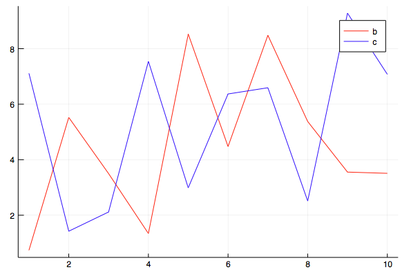
The last line of @df is the macro, df is the name of the variable with the DataFrame.
Query.jl can be a very useful library. Using the mechanisms of macros and channel processing, Query.jl provides a specialized query language. Example - get a list of persons over 50 and the number of children they have:
julia> using Query, DataFrames
julia> df = DataFrame(name=["John", "Sally", "Kirk"], age=[23., 42., 59.], children=[3,5,2])
3×3 DataFrame
│ Row │ name   │ age     │ children │
│     │ String │ Float64 │ Int64    │
├─────┼────────┼─────────┼──────────┤
│ 1   │ John   │ 23.0    │ 3        │
│ 2   │ Sally  │ 42.0    │ 5        │
│ 3   │ Kirk   │ 59.0    │ 2        │
julia> x = @from i in df begin
           @where i.age>50
           @select {i.name, i.children}
           @collect DataFrame
       end1×2 DataFrame
│ Row │ name   │ children │
│     │ String │ Int64    │
├─────┼────────┼──────────┤
│ 1   │ Kirk   │ 2        │
Or a form with a channel:
julia> using Query, DataFrames
julia> df = DataFrame(name=["John", "Sally", "Kirk"], age=[23., 42., 59.], children=[3,5,2]);
julia> x = df |> @query(i, begin
                   @where i.age>50
                   @select {i.name, i.children}
                 end) |> DataFrame
1×2 DataFrame
│ Row │ name   │ children │
│     │ String │ Int64    │
├─────┼────────┼──────────┤
│ 1 │ Kirk │ 2 │Both examples above demonstrate the use of query languages functionally similar to dplyr or LINQ. And these languages are not limited to Query.jl. Learn more about using these languages with DataFrames here .
The last example uses the “|>” operator. See more details .
This operator substitutes the argument in the function that is specified to the right of it. In other words:
julia> [1:5;] |> x->x.^2 |> sum |> inv
0.01818181818181818
Equivalent to:
julia> inv(sum( [1:5;] .^ 2 ))
0.01818181818181818
And the last thing I would like to note is the ability to write the DataFrame to the output format with a separator using the previously mentioned CSV.jl library
julia> df = DataFrame(name=["John", "Sally", "Kirk"], age=[23., 42., 59.], children=[3,5,2])
3×3 DataFrame
│ Row │ name   │ age     │ children │
│     │ String │ Float64 │ Int64    │
├─────┼────────┼─────────┼──────────┤
│ 1   │ John   │ 23.0    │ 3        │
│ 2   │ Sally  │ 42.0    │ 5        │
│ 3   │ Kirk   │ 59.0    │ 2        │
julia> CSV.write("out.csv", df)
"out.csv"
We can check the recorded result:
> catout.csvname,age,childrenJohn,23.0,3
Sally,42.0,5
Kirk,59.0,2
Conclusion
It is difficult to predict whether Julia will become a common programming language like R, for example, but this year it has already become the fastest growing programming language. If only a few people knew about it last year, this year, after the release of version 1.0 and the stabilization of library functions, they started writing about it, almost surely next year it will become a language that it’s simply not indecent in Data Science. And companies that have not started using Julia for data analysis will be outright dinosaurs to be replaced by more agile descendants.
Julia is a young programming language. Actually, after the appearance of pilot projects, it will be clear how ready Julia’s infrastructure is for real industrial use. Julia developers are very ambitious and declare readiness right now. In any case, the simple but strict Julia syntax makes it a very attractive programming language for learning now. High performance allows you to implement algorithms that are suitable not only for educational purposes, but also for real use in data analysis. We will begin to consistently try Julia in various projects now.