In simple words about a particle filter
In this article, I will tell you about one of the methods of optimal filtering - the Particle Filter - and show that applying such a filter is much easier than you think.
Optimal filtering
Optimal filtering algorithms are used in the calculation of systems affected by random processes. These algorithms make it possible to obtain an estimate of the system state parameters with a minimum standard deviation.
Particle filter
Particle filtering is one of the most popular optimal filtering methods. This method was used on a stand-alone Stanford Junior car, which took second place at the DARPA Challenge in 2007.
The particle filter allows you to get an estimate (approximate value) of the parameters of the system or object (we denote them as parameters A) which cannot be measured directly. To build this estimate, the filter uses measurements of other parameters (parameters B) associated with the former. We show this in the diagram:
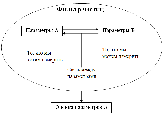
To evaluate the parameters A, the filter creates many hypotheses (particles) about the current value of these parameters. At the initial time, these hypotheses are completely random, but at each iteration of the filtering cycle, the filter will remove hypotheses that will not pass a validation test based on measurements of B.
Thus, from the set of hypotheses in the end, only those that are closest to the true value of the parameters A will remain.
This article considers one of the simplest applications of the particle filter. The robot moves in two-dimensional space and can measure the distance to certain objects in this space (landmarks). The task is to determine the location (coordinates) of the robot.
In this case, the robot can make turns with an accuracy of ± 5 degrees (turn error), move with an accuracy of ± 20 meters (movement error) and measure the distance to landmarks with an accuracy of ± 15 meters.
The particle filter algorithm is divided into two parts: initialization and the main filtering cycle.
Initialization
Before proceeding with filtering, the particle filter must be initialized - set parameters, initial distribution and other conditions of the filter.
The main parameter of the particle filter is the number of these particles (we denote this number N). Everything is simple here: the more particles, the more accurate the filter, and the more calculations you need to perform at each iteration of the main loop.
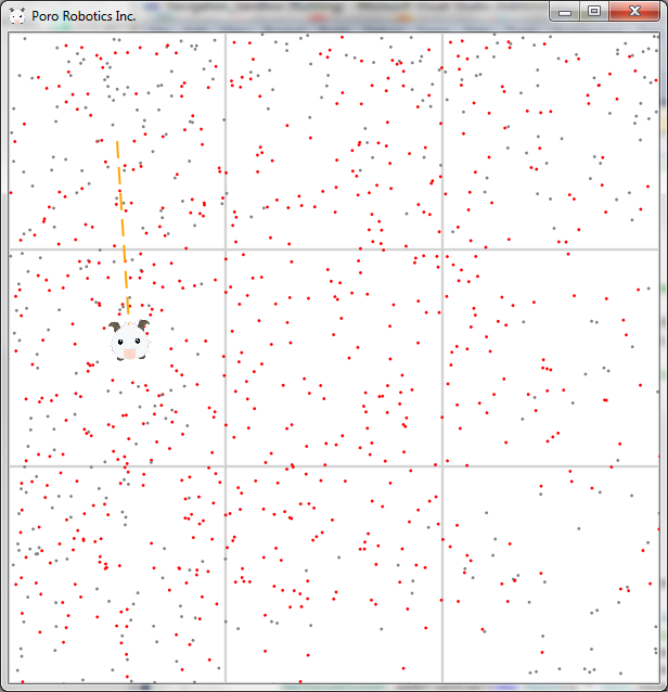
The initial distribution of particles depends on a priori information. For example, if we know that the robot is in a cell with coordinates (0, 0), then all particles must be randomly distributed inside this cell. (Click on image to enlarge.)
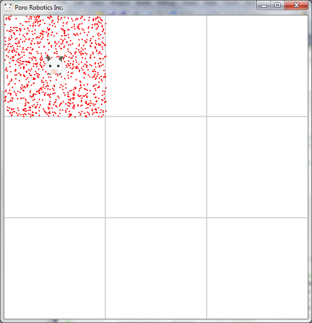
Moreover, the orientation of the robot (in the figures the robot is presented in the form of a little animal) inside this cell is unknown to us, therefore the orientation of each particle is random (from -180 to 180 degrees).
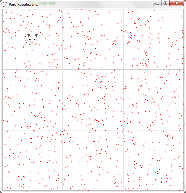
If there is no a priori information, then the particles are randomly distributed throughout the map. The main parameter of each particle is its weight. Particle weight determines the probability that the coordinates of this particle coincide with the coordinates of the robot. Since we assume that the full set of particles describes the position of our robot, the total weight of all particles is unity (this means that the robot is inside the area covered by all particles). In this case, regardless of the availability of a priori information, the weight of all particles at the initial moment of time should be the same and equal to 1 / N.
Also, at the initialization stage, restrictions should be imposed on the movement of particles (if any). In this example, particles have only one limitation - if a particle goes beyond the map, its weight becomes equal to zero.
If you have a map of the area, then on this map are marked the landmarks relative to which we will take measurements. These guidelines also need to be added to the particle filter. (It is possible to use a filter without a known map of the area and location of landmarks, but this is a topic for another article.)
In this example, four landmarks are used located at the corners of the map (they are not indicated in the figures).
Main filtering cycle
The main filtration cycle is divided into three phases:
Motion (Motion update)
At this stage, the robot makes a movement and, since the robot moves with errors, loses information about its location.
I will explain about the loss of information:
Suppose you stand still and know your geographical coordinates exactly. Then you take 100 steps forward. Since you are not a robot, and you cannot take 100 steps of the same length, you cannot determine the distance that you will cover these 100 steps (however, even if you were a robot, you would still have a movement error). Therefore, when you stop again you will know your coordinates only approximately.
Thus, having made the movement, you switched from “I know exactly where I am” to “I roughly know where I am” - that is, you lost information.
Since each particle is a model of a robot, then it should move like a robot. For example, if you give the robot the command "drive forward 200 meters," then all the particles should receive exactly the same command. Moreover, since the orientation of all particles is different, the “forward” of them is also different.
The calculation of the new coordinates of the robot is quite simple:
First, turn the robot at a given angle, simply adding the value of this angle to the current orientation of the robot:
Orientation = Orientation + angle
Then we calculate the new coordinates from pure trigonometry:
newX = oldX - distance * Sin(Orientation)
newY = oldY + distance * Cos(Orientation)
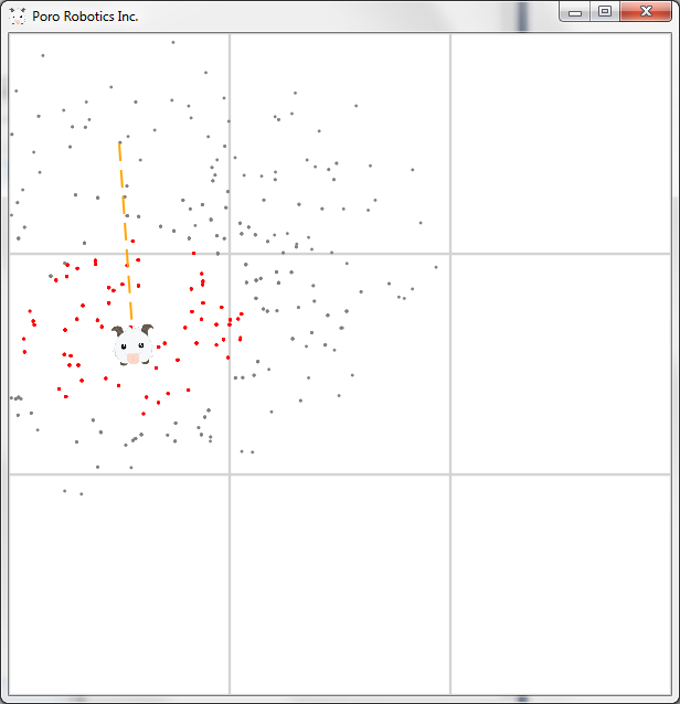
In this example, the zero rotation angle of the robot corresponds to the downward direction, and the angle of ninety degrees corresponds to the leftward direction. The figure shows that after the movement of the robot, the particle distribution has shifted. At the same time, particles with a low weight turned gray - these particles are still involved in the evaluation and the color change of the particles is made solely for clarity. We also note that due to the error in the rotation, the robot did not drive vertically down, but deviated by 3.7 degrees. The error of movement led to the fact that the robot did not pass 200 meters, but 185.
Do not forget that each particle is a model of the robot, and its movement also occurs with an error. At the same time, despite the fact that the model of particle errors is exactly the same as the model of robot errors, the actual error (the error obtained on the executed movement, in the given example is 3.7 degrees and 15 meters, respectively) of the particle’s movement does not depend on the actual robot error.
Measurement update
At this stage, the robot takes measurements and receives new information about its location.
Let us supplement the previous example, when we took 100 steps and lost information:
By measuring your coordinates at a new point, you go from “I know where I am approximately” to “I know exactly where I am again” - that is, you get information.
The physics of the measurements is not important, the main thing is that these measurements allow you to clarify the parameters that you evaluate by the particle filter.
In this example, the distance to the landmark is measured with a measurement error (± 15 meters). So far, everything is simple: we take measurements for the robot and for all particles.
The formula for calculating the distance to the landmark:
measurement = Sqrt((orientierX - robotX)^2 + (orientierY - robotY)^2)
Now we need to compare the measurements made by each particle with the measurements made by the robot in order to determine the weight of each particle.
For comparison, the measurement will use the normal distribution formula:
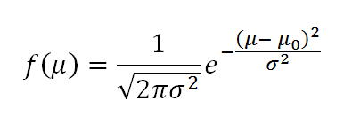 ,
, where σ ^ 2- standard deviation (measurement error); μ0 - mathematical expectation (measurement of the robot); μ is the value of the quantity (particle measurement); f (μ) is the probability of obtaining the value of μ for given μ0 and σ ^ 2.
If you use more than one reference point (and in most cases it is), then to calculate the particle weight you just need to multiply the probabilities of the measurements made. In this example, there are four guidelines and the particle weight is determined as follows:
particleList[i].weight = f(measurement[i][0]) * f(measurement[i][1]) * f(measurement[i][2]) * f(measurement[i][3])
Excellent! We processed the information received and calculated the weight of each particle. But now the total weight of all particles exceeds unity, which means it needs to be normalized (recall that the total weight of the particles should be 1).
S = Sum(weight)
for i in range(N):
	weight[i] = weight[i]/S
Now the total particle weight is equal to one and we can go to the last step of the filtration cycle.
Screening (Resampling)
Screening is needed in order to screen out particles with low weight, because they, in fact, are dead weight. The weight of the screened particles is small, which means that the likelihood of the location of the robot next to these particles is negligible. So why should we further model the motion and measurements of these particles, if we have already decided that they do not correspond to the position of the robot, it will be much more efficient to replace them with new particles that will increase the accuracy of assessing the state of the object (in this example, the coordinates of the robot).
The essence of the screening is to make a new array of N particles from an array of N particles, which will include only the particles with the largest weight. To be more precise, each particle from the first array goes into the second (undergoing screening) with a probability equal to its weight.
Example:
If the particle weight is equal to 0.0001, and the number of particles is N = 1000, then the probability that this particle will survive screening is:
1 - (1 - 0.0001)^1000 = 0.095 = 9.5 %
If the particle weight is equal to 0.005 (I recall that the initial weight of all particles was 1 / N = 0.001), then the probability that it will survive screening is:
1 - (1 - 0.005)^1000 = 0.993 = 99.3 %
There are many ways to apply such a dropout algorithm, but I will talk about one of the simplest and most effective - the Resampling wheel.
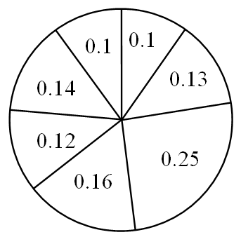
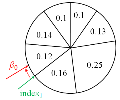
Consider this algorithm as an example. Take an array of seven particles (N = 7), and represent their weight as follows:
The algorithm starts with a random particle, so we take a random variable:
index = random.randint(0, 6) # index0
And we introduce the variable β equal to zero.
betta = 0
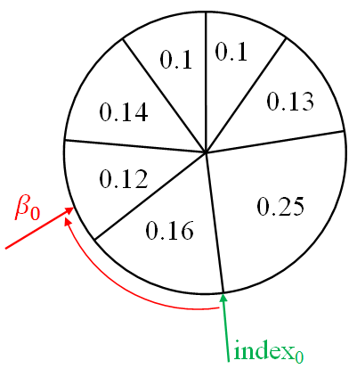
Now we add to β a random number from zero to twice the maximum weight (in this case, the maximum weight is 0.25):
betta = betta + random.uniform(0, 2*max(weight)) # betta0
After that, we compare the value of β with the value of the weight of the current particle. If β is greater than the particle weight, then we subtract the particle weight from β and increase the index by 1:
if betta > weight[index]:
	betta = betta - weight[index]
	index = index + 1
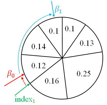
As soon as β becomes less than the weight of a particle, we add a copy of this particle to a new array of particles, return to the beginning of the cycle and increase β by a random number from zero to twice the maximum weight.
newParticleList.append(particleList[index])
betta = betta + random.uniform(0, 2*max(weight)) # betta1
Full screening algorithm code:
index = random.randint(0, 6)
betta = 0
for i in range(N):
	betta = betta + random.uniform(0, 2*max(weight))
	while betta > weight[index]:
		betta = betta - weight[index]
		index = (index + 1)%N # индекс изменяется в цикле от 0 до N
	newParticleList.append(particleList[index])
particleList = newParticleList
Thus, each particle goes into a new array with a probability equal to its weight, and can be added to the new array several times. After screening, it is necessary to normalize the particle weight again:
S = Sum(weight)
for i in range(N):
	weight[i] = weight[i]/S
Screening at each iteration of the filtration cycle is not necessary, but it is highly recommended at the first iterations - this will allow you to quickly filter out unnecessary particles (especially in the absence of a priori information) and get an accurate estimate. After this, screening can be done at regular intervals, for example, after each 20th or 100th iteration.
After the first screening, the particle distribution in the example will look like this:
Obtaining an assessment of the state of an object
You can get an assessment of the state of an object from a particle filter regardless of what phase it is currently in. To do this, it suffices to sum the value of the parameters of all particles multiplied by their weight:
estimateX = 0
estimateY = 0
for i in range(N):
	estimateX = estimateX + particleList[i].X*particleList[i].weight
	estimateY = estimateY + particleList[i].Y*particleList[i].weight
The result of the particle filter:
Conclusion
By using the particle filter in the above example, we managed to get the robot coordinates with an accuracy of 12.9 meters in just 8 iterations of the main cycle, with an error of movement of 20 meters and an error of measurement of 15 meters.
Having familiarized yourself with the basic principles of constructing a particle filter, you can now apply it to solve your own problems!
Related Links
Lecture Course on Autonomous Navigation Systems
Another example of a Stanford Junior particle filter implementation