FPGA Chaos Generators
Hello!
This article focuses on amazing features in the world of chaos. I will try to talk about how to curb such a strange and complex thing as a chaotic process and learn how to create my own simple chaos generators. Together with you, we will go from a dry theory to a beautiful visualization of chaotic processes in space. In particular, using the example of well-known chaotic attractors, I will show how to create dynamic systems and use them in problems associated with programmable logic integrated circuits (FPGAs).
Chaos theory- An unusual and young science that describes the behavior of nonlinear dynamical systems. In the process of its inception, the theory of chaos simply turned over modern science! She excited the minds of scientists and made them more and more immersed in the study of chaos and its properties. Unlike noise, which is a random process, chaos is deterministic. That is, for chaos, there is a law of variation of quantities included in the equations for describing a chaotic process. It would seem that with such a definition, chaos is no different from any other oscillations described as a function. But this is not so. Chaotic systems are very sensitive to initial conditions, and the slightest changes can lead to enormous differences. These differences can be so strong that it will not be possible to say if one or several systems were investigated.butterfly effect. "Many people heard about it, and even read books and watched movies that used the butterfly effect technique. In essence, the butterfly effect reflects the main property of chaos.
American scientist Edward Lorenz, one of the pioneers in the field of chaos, once said :

So, we will plunge into the theory of chaos and see what improvised means can generate chaos.
Before presenting the main material, I would like to give some definitions that will help to understand and clarify some points in the article.
A dynamic system is a certain set of elements for which a functional relationship between the time coordinate and the position in the phase space of each element of the system is given. Simply put, a dynamic system is a system in which the state in space changes over time.
Many physical processes in nature are described by systems of equations, which are dynamic systems. For example, these are the processes of combustion, the flow of liquids and gases, the behavior of magnetic fields and electrical vibrations, chemical reactions, meteorological phenomena, changes in populations of plants and animals, turbulence in sea currents, the movement of planets and even galaxies. As you can see, many physical phenomena can be described to one degree or another as a chaotic process.
A phase portrait is a coordinate plane in which each point corresponds to a state of a dynamical system at a particular moment in time. In other words, this is a spatial model of the system (it can be two-dimensional, three-dimensional, or even four-dimensional or more).
Attractor- a certain set of phase space of a dynamic system for which all trajectories are attracted to this set over time. If in a very simple language, then this is some area in which the behavior of the system in space is concentrated. Many chaotic processes are attractors, because they are concentrated in a certain area of space.
In this article I would like to talk about four main attractors - Lorentz, Rössler, Rikitake and Nose-Hoover. In addition to the theoretical description, the article reflects aspects of creating dynamic systems in MATLAB Simulink and their further integration into Xilinx FPGAs using the System Generator tool . Why not VHDL / Verilog? Attractors can also be synthesized using RTL languages, but for a better visualization of all processes, MATLAB is an ideal option. I will not touch on the difficult points associated with calculating the spectrum of Lyapunov exponents or constructing Poincare sections. And even more so, there will be no cumbersome mathematical formulas and conclusions. So let's get started.
To create chaos generators, we need the following software:
These programs are quite heavy, so be patient when installing them. It is better to start the installation with MATLAB, and then install the Xilinx software (with a different sequence, some of my friends could not integrate one application into another). When installing the latter, a window pops up where you can link Simulink and System Generator. There is nothing complicated and unusual in the installation, so this process is omitted.
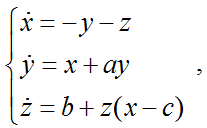
The Lorenz attractor is perhaps the most famous dynamical system in chaos theory. For several decades, he has attracted much attention of many researchers for the description of various physical processes. The first mention of the attractor is given in 1963 in the works of E. Lorenz, who was engaged in modeling atmospheric phenomena. The Lorenz attractor is a three-dimensional dynamical system of nonlinear autonomous differential equations of the first order. It has a complex topological structure, is asymptotically stable and Lyapunov stable. The Lorenz attractor is described by the following system of differential equations:

In the formula, a dot over the parameter means taking the derivative, which reflects the rate of change of the quantity with time (the physical meaning of the derivative).
With the parameter values σ = 10, r = 28, and b = 8/3, this simple dynamical system was obtained by E. Lorentz. For a long time he could not understand what was happening with his computer until he finally realized that the system was exhibiting chaotic properties! It was obtained in the course of experiments for the problem of simulating fluid convection. In addition, this dynamic system describes the behavior of the following physical processes:
The following figure shows the Lorenz attractor system in MATLAB:
The following notation is used in the figure:
In addition, the diagram shows auxiliary analysis tools, these are:
Inside each node of mathematical operations, it is necessary to indicate the length of the intermediate data and their type. Unfortunately, it is not so easy to work with FPGAs with a floating point, and in most cases all operations are performed in a fixed-point format. Incorrect setting of parameters can lead to incorrect results and upset you when building your systems. I experimented with different values, but settled on the following data type: 32-bit vector of signed numbers in a fixed-point format. 12 bits are allocated to the integer part, 20 bits to the fractional part.
Having set the initial value of the system in the integrators X, Y, Z in the trigger block, for example, {10, 0, 0} , I launched the model. In the time base, you can observe the following three signals:
Even if the modeling time goes to infinity, then the realization in time will never be repeated. Chaotic processes are non-periodic.
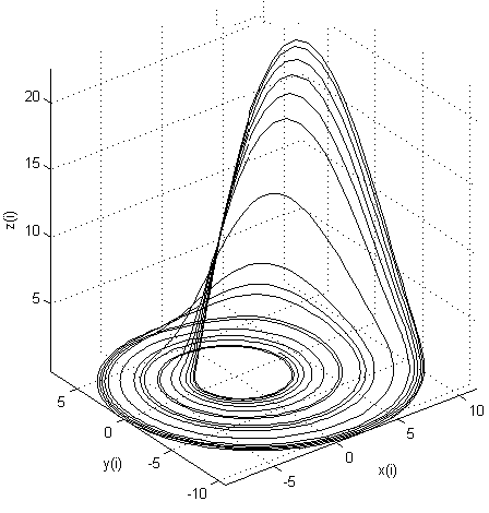
In three-dimensional space, the Lorenz attractor is as follows:

It can be seen that the attractor has two points of attraction around which the whole process takes place. With a slight change in the initial conditions, the process will also be concentrated around these points, but its trajectories will differ significantly from the previous version.
The second largest attractor in scientific articles and publications. The Rössler attractor is characterized by the presence of a boundary point of manifestation of chaotic or periodic properties. With certain parameters of the dynamic system, the oscillations cease to be periodic, and chaotic oscillations arise. One of the remarkable properties of the Rössler attractor is the fractal structure in the phase plane, that is, the phenomenon of self-similarity. It can be noted that other attractors, as a rule, possess this property.
The Rössler attractor is observed in many systems. For example, it is used to describe fluid flows, as well as to describe the behavior of various chemical reactions and molecular processes. The Rössler system is described by the following differential equations:
In MATLAB, an attractor is constructed as follows:
Temporal realization of spatial quantities:
Three-dimensional model of the Rössler attractor:
Compare the pictures of three-dimensional attractors under different initial conditions and coefficients in the system of equations. See how drastically the trajectories changed in the first case? But anyway, they are concentrated near a single area of attraction. In the second case, the attractor generally ceased to show signs of chaos, turning into a closed periodic loop (limit cycle).
Dynamo Rikitake is one of the well-known third-order dynamical systems with chaotic behavior. It is a model of a double-disk dynamo and was first proposed in problems of chaotic inversion of the Earth's geomagnetic field. The scientist Rikitake investigated a dynamo system with two interconnected disks constructed in such a way that the current from one disk coil flowed to another and excited the second disk, and vice versa. At some point, the system began to crash and show unpredictable things. Active studies of the attractor made it possible to project the Rikitake dynamo onto a model for coupling large eddies of magnetic fields in the Earth's core.
Dynamo Rikitake is described by the following system of equations:

Dynamo Rikitake model in MATLAB:
Temporary implementation:
Attractor (first version):

You may notice that the Rikitake dynamo is somewhat similar to the Lorenz attractor, but these are completely different systems and describe different physical processes!
A less famous, but no less important three-dimensional dynamic system is the Nose-Hoover thermostat . It is used in molecular theory as a time-reversible thermostatic system. Unfortunately, I know not so much about this attractor as about the others, but it seemed interesting to me and I included it in the review.
The Nose-Hoover thermostat is described by the following system of equations:
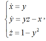
The Nose-Hoover model in MATLAB:
Temporary implementation:

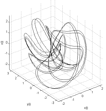
Two-dimensional projection of the attractor:

Three-dimensional model of the Nose-Hoover thermostat:
To synthesize the project, you need to click on the red “X” icon, which will launch the System Generator settings. Here you can choose the family and type of FPGAs, the resulting file format (VHDL / Verilog for creating source codes, NGC for creating a kernel as a list of connections), preliminary values of clock frequencies, etc. My typical settings are presented in the following figure:

After setting all the settings - click "Generate" and at the output we have a synthesized project for FPGAs. Next, it’s up to you to insert the generated kernel into the part of the project you need. (You can find how to do this in my other articles on digital signal processing). All of these attractors occupy very few resources in modern FPGAs (about 10-20 DSP48 blocks and a bit of logic).
The listed attractors are used in many physical processes in various fields of science and technology - from physics and chemistry to mechanics and meteorology. In particular, chaos generators are used to create long sequences of pseudorandom numbers (PSPs). In radio engineering problems, chaos can be used to modulate the carrier when creating ultra-wideband signals using digital methods (on FPGAs or processors).
Chaos Theory is an interesting and amazing science. And thanks to modern means of analysis and modeling, it becomes quite attractive for research. With the help of this article you can independently model your own dynamic systems, up to hyperchaotic systems of order higher than 3 (for example, hyperchaos of Lorentz, Rossler, etc.). I hope that the material of my publication may be useful to someone, but someone will find something new and useful for themselves.
Github Attractor Source Files
My articles on similar topics:
Hurray, the FPGA hub has returned to the hub Happy New Year, everyone!
This article focuses on amazing features in the world of chaos. I will try to talk about how to curb such a strange and complex thing as a chaotic process and learn how to create my own simple chaos generators. Together with you, we will go from a dry theory to a beautiful visualization of chaotic processes in space. In particular, using the example of well-known chaotic attractors, I will show how to create dynamic systems and use them in problems associated with programmable logic integrated circuits (FPGAs).
Introduction
Chaos theory- An unusual and young science that describes the behavior of nonlinear dynamical systems. In the process of its inception, the theory of chaos simply turned over modern science! She excited the minds of scientists and made them more and more immersed in the study of chaos and its properties. Unlike noise, which is a random process, chaos is deterministic. That is, for chaos, there is a law of variation of quantities included in the equations for describing a chaotic process. It would seem that with such a definition, chaos is no different from any other oscillations described as a function. But this is not so. Chaotic systems are very sensitive to initial conditions, and the slightest changes can lead to enormous differences. These differences can be so strong that it will not be possible to say if one or several systems were investigated.butterfly effect. "Many people heard about it, and even read books and watched movies that used the butterfly effect technique. In essence, the butterfly effect reflects the main property of chaos.
American scientist Edward Lorenz, one of the pioneers in the field of chaos, once said :
A butterfly flapping its wings in Iowa can trigger an avalanche of effects that culminate in the rainy season in Indonesia.
So, we will plunge into the theory of chaos and see what improvised means can generate chaos.
Theory
Before presenting the main material, I would like to give some definitions that will help to understand and clarify some points in the article.
A dynamic system is a certain set of elements for which a functional relationship between the time coordinate and the position in the phase space of each element of the system is given. Simply put, a dynamic system is a system in which the state in space changes over time.
Many physical processes in nature are described by systems of equations, which are dynamic systems. For example, these are the processes of combustion, the flow of liquids and gases, the behavior of magnetic fields and electrical vibrations, chemical reactions, meteorological phenomena, changes in populations of plants and animals, turbulence in sea currents, the movement of planets and even galaxies. As you can see, many physical phenomena can be described to one degree or another as a chaotic process.
A phase portrait is a coordinate plane in which each point corresponds to a state of a dynamical system at a particular moment in time. In other words, this is a spatial model of the system (it can be two-dimensional, three-dimensional, or even four-dimensional or more).
Attractor- a certain set of phase space of a dynamic system for which all trajectories are attracted to this set over time. If in a very simple language, then this is some area in which the behavior of the system in space is concentrated. Many chaotic processes are attractors, because they are concentrated in a certain area of space.
Implementation
In this article I would like to talk about four main attractors - Lorentz, Rössler, Rikitake and Nose-Hoover. In addition to the theoretical description, the article reflects aspects of creating dynamic systems in MATLAB Simulink and their further integration into Xilinx FPGAs using the System Generator tool . Why not VHDL / Verilog? Attractors can also be synthesized using RTL languages, but for a better visualization of all processes, MATLAB is an ideal option. I will not touch on the difficult points associated with calculating the spectrum of Lyapunov exponents or constructing Poincare sections. And even more so, there will be no cumbersome mathematical formulas and conclusions. So let's get started.
To create chaos generators, we need the following software:
- MATLAB R2014 licensed for Simulink and DSP Toolbox.
- Xilinx ISE Design Suite 14.7 licensed System-Generator (DSP Edition)
These programs are quite heavy, so be patient when installing them. It is better to start the installation with MATLAB, and then install the Xilinx software (with a different sequence, some of my friends could not integrate one application into another). When installing the latter, a window pops up where you can link Simulink and System Generator. There is nothing complicated and unusual in the installation, so this process is omitted.
Attractor Lorenz
The Lorenz attractor is perhaps the most famous dynamical system in chaos theory. For several decades, he has attracted much attention of many researchers for the description of various physical processes. The first mention of the attractor is given in 1963 in the works of E. Lorenz, who was engaged in modeling atmospheric phenomena. The Lorenz attractor is a three-dimensional dynamical system of nonlinear autonomous differential equations of the first order. It has a complex topological structure, is asymptotically stable and Lyapunov stable. The Lorenz attractor is described by the following system of differential equations:
In the formula, a dot over the parameter means taking the derivative, which reflects the rate of change of the quantity with time (the physical meaning of the derivative).
With the parameter values σ = 10, r = 28, and b = 8/3, this simple dynamical system was obtained by E. Lorentz. For a long time he could not understand what was happening with his computer until he finally realized that the system was exhibiting chaotic properties! It was obtained in the course of experiments for the problem of simulating fluid convection. In addition, this dynamic system describes the behavior of the following physical processes:
- - model of a single-mode laser,
- - convection in a closed loop and a flat layer,
- - rotation of the water wheel,
- - harmonic oscillator with inertial nonlinearity,
- - turbulence of cloud masses, etc.
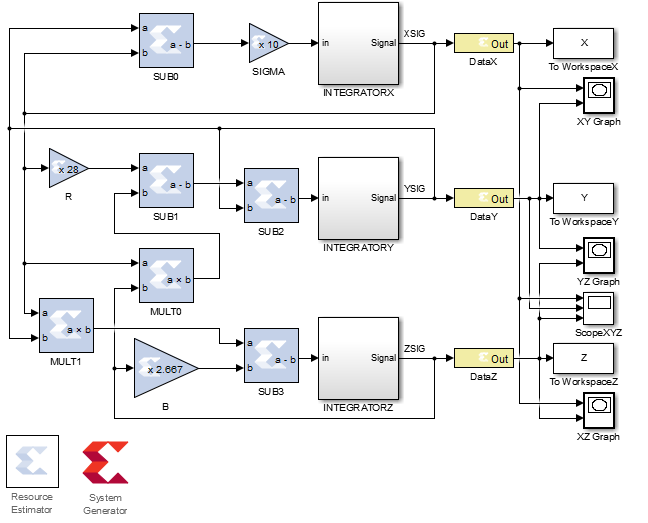
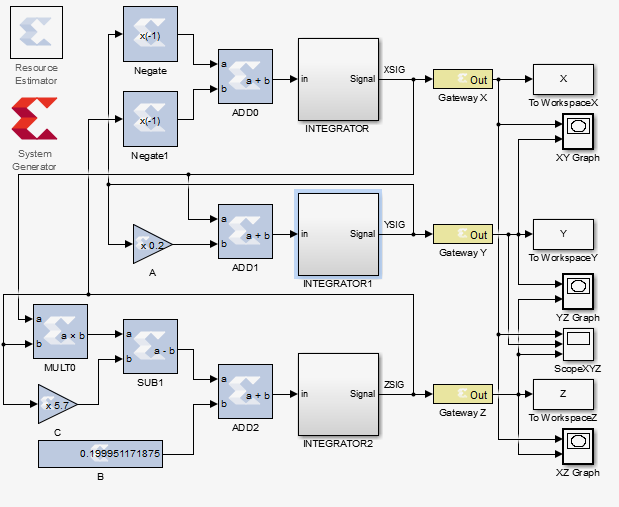
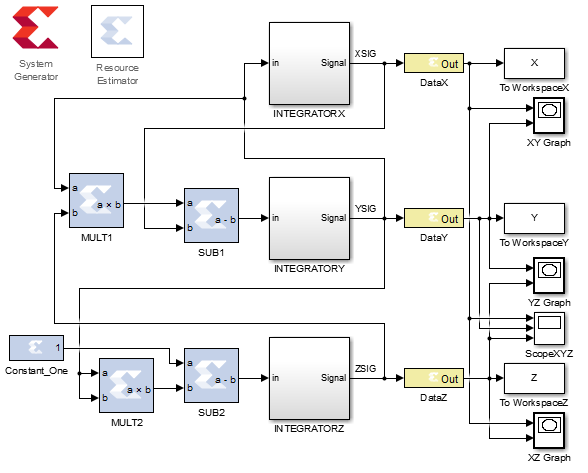
The following figure shows the Lorenz attractor system in MATLAB:
The following notation is used in the figure:
- Subtractors : SUB0-3 ;
- constant multipliers: SIGMA, B, R ;
- multipliers: MULT0-1 ;
- integrators with a cell for setting the initial condition: INTEGRATOR X, Y, Z ;
- OUT output ports: DATA X, Y, Z for XSIG, YSIG, ZSIG signals ;
In addition, the diagram shows auxiliary analysis tools, these are:
- saving calculation results to a file: To Workspace X, Y, Z ;
- spatial graphing: Graph XY, YZ, XZ ;
- plotting timelines: Scope XYZ ;
- tools for assessing the occupied resources of the crystal and generating HDL code from the Resource Estimator and System Generator models .
Inside each node of mathematical operations, it is necessary to indicate the length of the intermediate data and their type. Unfortunately, it is not so easy to work with FPGAs with a floating point, and in most cases all operations are performed in a fixed-point format. Incorrect setting of parameters can lead to incorrect results and upset you when building your systems. I experimented with different values, but settled on the following data type: 32-bit vector of signed numbers in a fixed-point format. 12 bits are allocated to the integer part, 20 bits to the fractional part.
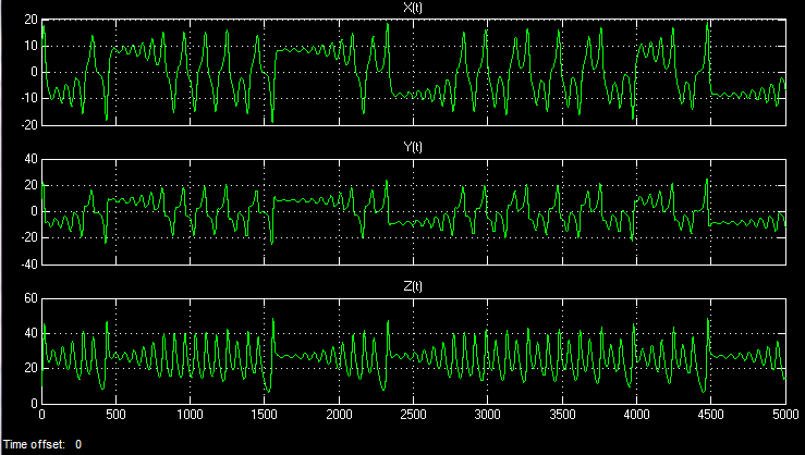
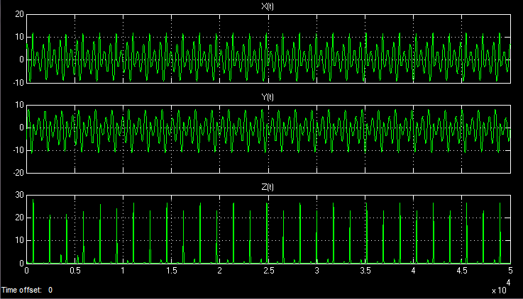
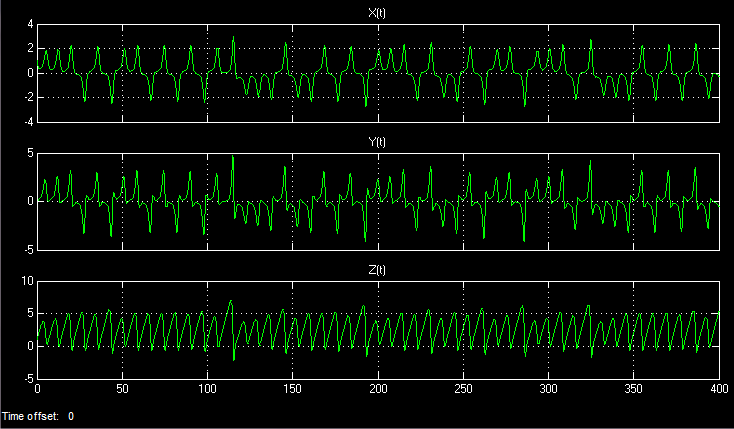
Having set the initial value of the system in the integrators X, Y, Z in the trigger block, for example, {10, 0, 0} , I launched the model. In the time base, you can observe the following three signals:
Even if the modeling time goes to infinity, then the realization in time will never be repeated. Chaotic processes are non-periodic.
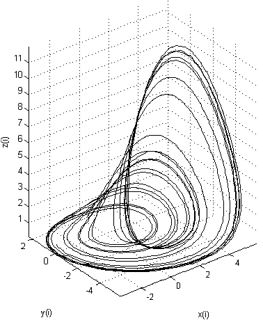
In three-dimensional space, the Lorenz attractor is as follows:
It can be seen that the attractor has two points of attraction around which the whole process takes place. With a slight change in the initial conditions, the process will also be concentrated around these points, but its trajectories will differ significantly from the previous version.
Rössler Attractor
The second largest attractor in scientific articles and publications. The Rössler attractor is characterized by the presence of a boundary point of manifestation of chaotic or periodic properties. With certain parameters of the dynamic system, the oscillations cease to be periodic, and chaotic oscillations arise. One of the remarkable properties of the Rössler attractor is the fractal structure in the phase plane, that is, the phenomenon of self-similarity. It can be noted that other attractors, as a rule, possess this property.
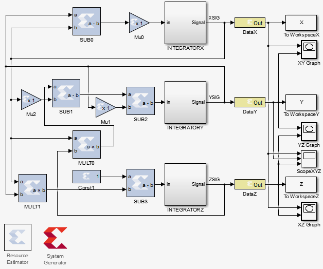
The Rössler attractor is observed in many systems. For example, it is used to describe fluid flows, as well as to describe the behavior of various chemical reactions and molecular processes. The Rössler system is described by the following differential equations:
In MATLAB, an attractor is constructed as follows:
Temporal realization of spatial quantities:
Three-dimensional model of the Rössler attractor:
Bam! The values have slightly changed:
Attractor with slightly changed initial conditions (the trajectories differ!)
Attractor with different coefficients in the system of equations (a chaotic process turned into a periodic one!)

Attractor with different coefficients in the system of equations (a chaotic process turned into a periodic one!)
Compare the pictures of three-dimensional attractors under different initial conditions and coefficients in the system of equations. See how drastically the trajectories changed in the first case? But anyway, they are concentrated near a single area of attraction. In the second case, the attractor generally ceased to show signs of chaos, turning into a closed periodic loop (limit cycle).
Attractor Rikitake
Dynamo Rikitake is one of the well-known third-order dynamical systems with chaotic behavior. It is a model of a double-disk dynamo and was first proposed in problems of chaotic inversion of the Earth's geomagnetic field. The scientist Rikitake investigated a dynamo system with two interconnected disks constructed in such a way that the current from one disk coil flowed to another and excited the second disk, and vice versa. At some point, the system began to crash and show unpredictable things. Active studies of the attractor made it possible to project the Rikitake dynamo onto a model for coupling large eddies of magnetic fields in the Earth's core.
Dynamo Rikitake is described by the following system of equations:
Dynamo Rikitake model in MATLAB:
Temporary implementation:
Attractor (first version):
Dynamo (second version)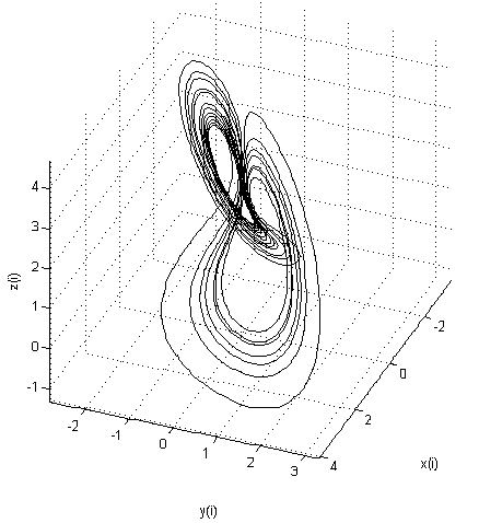
You may notice that the Rikitake dynamo is somewhat similar to the Lorenz attractor, but these are completely different systems and describe different physical processes!
Attractor Nose Hoover
A less famous, but no less important three-dimensional dynamic system is the Nose-Hoover thermostat . It is used in molecular theory as a time-reversible thermostatic system. Unfortunately, I know not so much about this attractor as about the others, but it seemed interesting to me and I included it in the review.
The Nose-Hoover thermostat is described by the following system of equations:
The Nose-Hoover model in MATLAB:
Temporary implementation:
Two-dimensional projection of the attractor:
Three-dimensional model of the Nose-Hoover thermostat:
Thermostat (second version)
Project Synthesis
To synthesize the project, you need to click on the red “X” icon, which will launch the System Generator settings. Here you can choose the family and type of FPGAs, the resulting file format (VHDL / Verilog for creating source codes, NGC for creating a kernel as a list of connections), preliminary values of clock frequencies, etc. My typical settings are presented in the following figure:
After setting all the settings - click "Generate" and at the output we have a synthesized project for FPGAs. Next, it’s up to you to insert the generated kernel into the part of the project you need. (You can find how to do this in my other articles on digital signal processing). All of these attractors occupy very few resources in modern FPGAs (about 10-20 DSP48 blocks and a bit of logic).
Life examples
The Lorenz attractor on the oscilloscope screen:

A galaxy system similar to the Lorentz attractor:
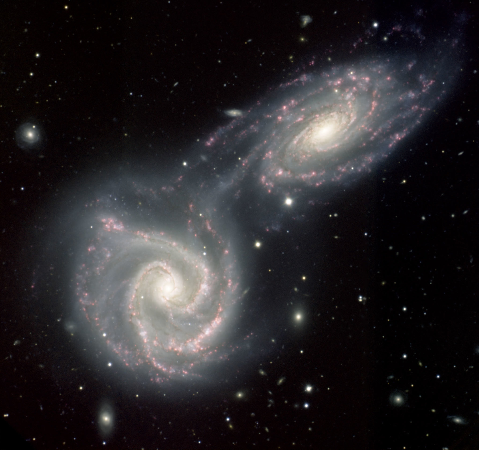
A galaxy system similar to the Lorentz attractor:
Conclusion
The listed attractors are used in many physical processes in various fields of science and technology - from physics and chemistry to mechanics and meteorology. In particular, chaos generators are used to create long sequences of pseudorandom numbers (PSPs). In radio engineering problems, chaos can be used to modulate the carrier when creating ultra-wideband signals using digital methods (on FPGAs or processors).
Chaos Theory is an interesting and amazing science. And thanks to modern means of analysis and modeling, it becomes quite attractive for research. With the help of this article you can independently model your own dynamic systems, up to hyperchaotic systems of order higher than 3 (for example, hyperchaos of Lorentz, Rossler, etc.). I hope that the material of my publication may be useful to someone, but someone will find something new and useful for themselves.
Github Attractor Source Files
My articles on similar topics:
Literature
- Chaos on the hub
- Chaoscope online
- Chaos. Creating a new science
- Chaos Theory - Wiki
- Attractor Lorenz - Wiki
- Rössler Attractor - Wiki
- Elegant Chaos (also sold in Russian)
Hurray, the FPGA hub has returned to the hub Happy New Year, everyone!