Evolution of data structures in Yandex.Metrica
Yandex.Metrica today is not only a web analytics system, but also AppMetrica - an analytics system for applications. At the entrance to Metrica, we have a stream of data - events that occur on sites or in applications. Our task is to process this data and present it in a form suitable for analysis.
But data processing is not a problem. The problem is how and in what form to save processing results so that you can conveniently work with them. During the development process, we had to completely change the approach to organizing data storage several times. We started with MyISAM tables, used LSM trees, and eventually came up with a column-oriented database. In this article I want to tell you what made us do this.

Yandex.Metrica has been working since 2008 - more than seven years. Each time, a change in the approach to data storage was due to the fact that one or another solution worked too poorly - with insufficient productivity margin, insufficiently reliable and with a lot of problems during operation, used too many computing resources, or simply did not allow us to implement that what we want.
In the old Metric for sites, there are about 40 “fixed” reports (for example, a report on the geography of visitors), several tools for in-page analytics (for example, a click map), Webvisor (which allows you to examine as much as possible the actions of individual visitors) and, separately, report constructor.
In the new Metric, and also in Appmetrica, instead of “fixed” reports, each report can be arbitrarily changed. You can add new dimensions (for example, in the report on search phrases add another breakdown on the pages of the site’s entrance), segment and compare (you can compare the sources of traffic to the site for all visitors and visitors from Moscow), change the set of metrics, and so on. Of course, this requires completely different approaches to data storage.
At the very beginning, Metric was created as part of Direct. In Yandex.Direct, MyISAM tables were used to solve the problem of storing statistics, and we also started from this. We used MyISAM to store “fixed” reports from 2008 to 2011.
Let me tell you what the table structure should be for reporting, for example, by geography. The report is shown for a specific site (more precisely, the Metric counter number). This means that the counter number must be included in the primary key - CounterID. The user can select an arbitrary reporting period. It would be unreasonable to save data for each pair of dates, therefore they are saved for each date and then, when requested, are summed for a given interval. That is, the primary key includes the date - Date.
The report displays data for the regions in the form of a tree from countries, regions, cities, or in the form of a list. It is reasonable to place the region identifier (RegionID) in the primary key of the table, and to collect data into the tree already on the side of the application code, not the database.
It is also considered, for example, the average duration of the visit. This means that the columns of the table should contain the number of visits and the total duration of visits.
As a result, the table structure is as follows: CounterID, Date, RegionID -> Visits, SumVisitTime, ... Consider what happens when we want to get a report. A request is made
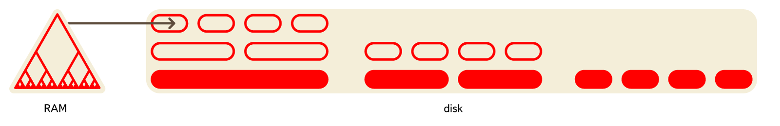
MyISAM table is a data file and a file with indexes. If nothing was deleted from the table and the lines did not change their length during the update, the data file will be serialized lines arranged in a row in the order they were added. The index (including the primary key) is a B-tree, in the leaves of which there are offsets in the data file. When we read data on an index range, a lot of offsets in the data file are extracted from the index. Then, readings from the data file are made over this set of offsets.
Suppose a natural situation is when the index is in RAM (key cache in MySQL or the system page cache), and the data is not cached in it. Suppose we use hard drives. The time for reading data depends on how much data you need to read and how many seeks you need to make. The number of seeks is determined by the locality of the location of the data on the disk.
Events in Metric arrive in an order almost corresponding to the time of events. In this incoming stream, the data of different counters are scattered in a completely arbitrary way. That is, incoming data is local in time, but not local in counter number. When writing to the MyISAM table, the data of different counters will also be located in a completely random manner, which means that to read the report data, it will be necessary to perform approximately as many random readings as there are rows we need in the table.
A regular 7200 RPM hard drive can perform from 100 to 200 random reads per second, and when used correctly, the RAID array is proportionally larger. One five-year-old SSD can do 30,000 random reads per second, but we cannot afford to store our data on an SSD. Thus, if you need to read 10,000 lines for our report, then it is unlikely to take less than 10 seconds, which is completely unacceptable.
InnoDB is better suited for reading over the primary key range, since InnoDB uses a clustered primary key (that is, data is stored in order by primary key). But InnoDB was impossible to use due to the low write speed. If reading this text, you remembered TokuDB , then continue to read this text.
In order for MyISAM to work faster when choosing a primary key for a range, some tricks were used.
Sort table . Since the data must be updated incrementally, it is not enough to sort the table once, and it is impossible to sort it every time. However, this can be done periodically for old data.
Partitioning. The table is divided into a number of smaller primary key ranges. At the same time, there is a hope that the data of one partition will be stored more or less locally, and requests for the range of the primary key will work faster. This method can be called “manual cluster primary key”. At the same time, data insertion slows down somewhat. Choosing the number of partitions, as a rule, it is possible to reach a compromise between the speed of inserts and readings.
Generating data. With one partitioning scheme, reads can be too slow, with another - inserts, and with an intermediate - both of them. In this case, data can be divided into several generations. For example, we call the first generation operational data - there partitioning is done in the insertion order (in time) or not at all. We will call the second generation archival data - there it is produced in the reading order (by counter number). Data is transferred from generation to generation by a script, but not too often (for example, once a day). Data is read immediately from all generations. This usually helps, but adds quite a bit of complexity.
All these tricks (and some others) were used in Yandex.Metrica long ago in order for everything to work somehow.
We summarize what are the disadvantages:
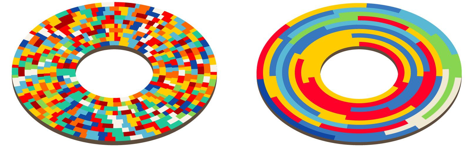
Locality of data on disk, figurative representation
In general, the use of MyISAM was extremely inconvenient. In the daytime, the servers worked with 100% load on disk arrays (constant head movement). Under such conditions, disks fail more often than usual. On the servers, we used disk shelves (16 disks) - that is, quite often we had to restore RAID arrays. At the same time, replication lagged even further and sometimes the replica had to be poured again. Switching the wizard is extremely inconvenient. To select the replica to which requests are sent, we used MySQL Proxy, and this use was very unsuccessful (then we replaced it with HAProxy).
Despite these shortcomings, as of 2011 we have stored more than 580 billion rows in MyISAM tables. Then everything was converted to Metrage, deleted, and as a result, many servers were freed.
We use Metrage to store fixed reports from 2010 to the present. Suppose you have the following work scenario:
A fairly common LSM-Tree data structure is well suited for this . It is a relatively small set of “pieces” of data on a disk, each of which contains data sorted by primary key. New data is first located in some data structure in RAM (MemTable), then it is written to disk in a new sorted piece. Periodically in the background, several sorted pieces are combined into one larger sorted (compaction). Thus, a relatively small set of pieces is constantly maintained.
Among the embedded data structures, LSM-Tree implements LevelDB , RocksDB . It is used in HBase and Cassandra .
Metrage is also an LSM-Tree. As "lines" in it arbitrary data structures can be used (fixed at the compilation stage). Each line is a key, value pair. The key is a structure with comparison operations for equality and inequality. Value - an arbitrary structure with the operations update (add something) and merge (aggregate, combine with another value). In short, this is CRDT .
The values can be either simple structures (a tuple of numbers) or more complex structures (a hash table for calculating the number of unique visitors, a structure for a click map). Using the update and merge operations, incremental data aggregation is constantly performed:
Metrage also contains the domain-specific logic we need, which is executed upon requests. For example, for reporting by region, the key in the table will contain the identifier of the lowest region (city, village), and if we need to get a report by country, then data will be aggregated to country data on the database server side.
I will list the advantages of this data structure:
Since readings are not performed very often, but they read quite a lot of lines, an increase in latency due to the presence of many pieces and uncleaning of the data block and reading of extra lines due to the sparseness of the index do not matter.
Recorded chunks of data are not modified. This allows you to read and write without locking - a snapshot of data is taken for reading. Simple and uniform code is used, but we can easily implement all the domain-specific logic we need.
We had to write Metrage instead of finalizing any existing solution, because there was no existing solution. For example, LevelDB did not exist in 2010. TokuDB at that time was available only for money.
All systems implementing the LSM-Tree were suitable for storing unstructured data and displaying the BLOB -> BLOB type with slight variations. Adapting this to working with arbitrary CRDTs would take a lot more time than developing Metrage.
Converting data from MySQL to Metrage was quite time-consuming: the pure time for the conversion program to work was only about a week, but the main part of the work was completed in only two months.
After translating the reports to Metrage, we immediately gained an advantage in the speed of the Metrica interface. Thus, the 90% percentile of the report loading time for page titles decreased from 26 seconds to 0.8 seconds (total time, including the operation of all database queries and subsequent data transformations). The processing time for requests from Metrage itself (for all reports) is: median - 6 ms, 90% - 31 ms, 99% - 334 ms.
We used Metrage for five years, and it has proven to be a reliable, trouble-free solution. For all the time there were only a few minor glitches. The advantages in efficiency and ease of use compared to storing data in MyISAM are dramatic.
We are now storing 3.37 trillion lines in Metrage. For this, 39 * 2 servers are used. We gradually refuse to store data in Metrage and have already deleted some of the largest tables. But this system also has a drawback - you can work effectively only with fixed reports. Metrage aggregates data and stores aggregated data. And in order to do this, you need to list in advance all the ways that we want to aggregate data. If we do this in 40 different ways, it means that there will be 40 reports in the Metric, but no more.
In Yandex.Metrica, the amount of data and the amount of load are large enough so that the main problem is to make a solution that at least works - solves the problem and at the same time copes with the load within an adequate amount of computing resources. Therefore, often the main effort is spent on creating a minimal working prototype.
One such prototype was OLAPServer. We used OLAPServer from 2009 to 2013 as a data structure for the report designer.
Our task is to receive arbitrary reports, the structure of which becomes known only at the moment when the user wants to receive a report. For this, it is impossible to use pre-aggregated data, because it is impossible to foresee all combinations of measurements, metrics, conditions in advance. So, you need to store non-aggregated data. For example, for reports calculated on the basis of visits, it is necessary to have a table where each visit will have a line, and each parameter by which the report can be calculated will have a column.
We have such a scenario:
For such a work scenario (let's call it an OLAP work scenario), column-oriented DBMSs are best suited . This is the name of the DBMS, in which data for each column is stored separately, and the data of one column is stored together.
Column-based DBMSs work effectively for the OLAP scenario for the following reasons:
1. By I / O.
For example, for the query “calculate the number of entries for each advertising system”, you need to read one column “Identifier of the advertising system”, which takes 1 byte in uncompressed form. If most of the transitions were not from advertising systems, then you can count on at least tenfold compression of this column. Using a fast compression algorithm, data can be compressed at a speed of more than several gigabytes of uncompressed data per second. That is, such a request can be executed at a speed of about several billion rows per second on a single server.

2. By CPU.
Since a sufficiently large number of lines must be processed to complete the request, it becomes relevant to dispatch all operations not for individual lines, but for entire vectors (for example, the vector engine in the VectorWise DBMS) or implement the query execution engine so that dispatching costs are approximately zero (for example, code generation using LLVM in Cloudera Impala ). If this is not done, then with any not too bad disk subsystem, the query interpreter will inevitably run into the CPU. It makes sense not only to store data in columns, but also to process them, if possible, also in columns.
There are many columnar DBMSs. This, for example, Vertica , Paraccel ( Actian Matrix ) ( Amazon Redshift ), Sybase IQ (SAP IQ), Exasol , Infobright , InfiniDB , MonetDB (VectorWise) ( Actian Vector ),LucidDB , SAP HANA , Google Dremel , Google PowerDrill , Metamarkets Druid , kdb + , etc.
In traditionally string DBMSs, too, recently began to appear solutions for storing data by columns. Examples are column store index in MS SQL Server , MemSQL , cstore_fdw for Postgres, ORC-File and Parquet formats for Hadoop.
OLAPServer is the simplest and most limited implementation of a column database. So OLAPServer supports only one table specified in compile time, a visit table. Updating data is not done in real time, like everywhere else in Metric, but several times a day. Only fixed-length numbers of 1-8 bytes are supported as data types. And as a request, only an option is supported
Despite such limited functionality, OLAPServer successfully coped with the task of the report designer. But I could not cope with the task of realizing the possibility of customizing each Yandex.Metrica report. For example, if the report contained URLs, then it could not be obtained through the report designer, because OLAPServer did not store URLs; it was not possible to implement the functionality often needed by our users - viewing login pages for search phrases.
As of 2013, we stored 728 billion lines in OLAPServer. Then all the data was transferred to ClickHouse and deleted.
Using OLAPServer, we managed to understand how well column-based DBMSs do ad-hoc analytics on non-aggregated data. If any report can be obtained from non-aggregated data, the question arises whether it is necessary to pre-aggregate the data in advance, how do we do it using Metrage?
On the one hand, data pre-aggregation reduces the amount of data used directly at the time of loading the report page. Aggregated data, on the other hand, is a very limited solution. The reasons are as follows:
As you can see, if you do not aggregate and work with non-aggregated data, it can even reduce the amount of computation. But working only with non-aggregated data imposes very high requirements on the efficiency of the system that will fulfill the requests.
So, if we aggregate the data in advance, then we do it though constantly (in real time), but asynchronously with respect to user requests. We just have to manage to aggregate the data in real time - at the time of receipt of the report, for the most part, prepared data are used.
If you do not aggregate the data in advance, then all the work needs to be done at the time of the user’s request - while he is waiting for the report page to load. This means that during a query, you may need to process many billions of lines, and the faster the better.
To do this, you need a good columnar DBMS. There is not a single columnar DBMS on the market that can work quite well on the tasks of Internet analytics on a Runet scale and at the same time have a prohibitively high cost of licenses. If we used some of the solutions listed in the previous section, the cost of licenses would be many times higher than the cost of all our servers and employees.
Recently, as an alternative to commercial columnar DBMS, solutions for effective ad-hoc analytics based on data found in distributed computing systems have appeared: Cloudera Impala , Spark SQL , Presto , Apache Drill . Although such systems can effectively work on requests for internal analytical tasks, it is rather difficult to imagine them as a backend for the web interface of the analytical system available to external users.
Yandex has developed its own column database - ClickHouse. Consider the basic requirements that we had to her before proceeding with the development.
Ability to work with big data.In the new Yandex.Metrica, ClickHouse is used to store all the data for reports. The volume of the database as of December 2015 was 11.4 trillion rows (and this is only for the big Metric). Rows are non-aggregated data that are used to receive real-time reports. Each row in the largest tables contains more than 200 columns.
The system must scale linearly.ClickHouse allows you to increase cluster size by adding new servers as needed. For example, the main cluster of Yandex.Metrica was increased from 60 to 394 servers in two years. For fault tolerance, servers are located in different data centers. ClickHouse can use all the features of iron to process a single request. This achieves a speed of more than 1 terabyte per second (data after decompression, only used columns).
High work efficiency.High base performance is our individual pride. According to the results of internal tests, ClickHouse processes requests faster than any other system that we could get. For example, ClickHouse is on average 2.8-3.4 times faster than Vertica. ClickHouse does not have a single silver bullet, due to which the system works so fast.
The functionality should be sufficient for web analytics tools. The base supports SQL dialect, subqueries and JOINs (local and distributed). There are numerous SQL extensions: functions for web analytics, arrays and nested data structures, higher-order functions, aggregate functions for approximate calculations using sketching, etc. When working with ClickHouse you get the convenience of a relational DBMS.
ClickHouse is developed in the Yandex.Metrica team. At the same time, the system was made flexible enough and extensible so that it can be successfully used for various tasks. Although the database can operate on large clusters, it can be installed on one server or even on a virtual machine. There are now more than a dozen ClickHouse applications within the company.
ClickHouse is well suited for creating all kinds of analytical tools. Indeed, if the system successfully copes with the tasks of big Yandex.Metrica, then you can be sure that ClickHouse will cope with multiple tasks in terms of other tasks.
In this sense, Appmetrica was especially lucky - when it was in development, ClickHouse was already ready. To process application analytics data, we just made one program that takes incoming data and after a little processing writes it to ClickHouse. Any functionality available in the Appmetrica interface is simply a SELECT query.
ClickHouse is used to store and analyze the logs of various services in Yandex. A typical solution would be to use Logstash and ElasticSearch, but it does not work on a more or less decent data stream.
ClickHouse is suitable as a database for time series - for example, in Yandex it is used as a backend for Graphiteinstead of ceres / whisper. This allows you to work with more than a trillion metrics on a single server.
ClickHouse uses analytics for internal tasks. According to the experience of using inside the company, ClickHouse's work efficiency is approximately three orders of magnitude higher than traditional data processing methods (MR scripts). This cannot be regarded as simply a quantitative difference. The fact is that having such a high calculation speed, you can afford fundamentally different methods for solving problems.
If the analyst got the task of making a report, and if he is a good analyst, then he will not do one report. Instead, he will first receive a dozen other reports in order to better study the nature of the data and test the hypotheses that arise. It often makes sense to look at the data from different angles, without even having any clear purpose, in order to find new hypotheses and test them.
This is only possible if the speed of data analysis allows you to conduct research in an interactive mode. The faster the queries are executed, the more hypotheses can be tested. When working with ClickHouse, it feels like you have increased your speed of thinking.
In traditional systems, the data, figuratively speaking, lie dead weight at the bottom of the swamp. You can do anything with them, but it will take a lot of time and will be very inconvenient. And if your data is in ClickHouse, then this is “live” data: you can study it in any slices and “drill” to each individual line.
It just so happened that Yandex.Metrica is the second largest web analytics system in the world. The volume of data received in Metrica increased from 200 million events per day in early 2009 to a little more than 20 billion in 2015. In order to give users quite rich opportunities, but at the same time not to stop working under an increasing load, we had to constantly change the approach to organizing data storage.
Efficiency of use of iron is very important for us. In our experience, with a large amount of data, you should not worry about how well the system scales well, but about how efficiently each unit of resources is used: each processor core, disk and SSD, RAM, network. After all, if your system already uses hundreds of servers, and you need to work ten times more efficiently, then you can hardly easily install thousands of servers, no matter how well the system scales.
To achieve maximum efficiency, specialization for a specific class of tasks is important. There is no data structure that handles completely different scenarios. For example, it is obvious that the key-value base is not suitable for analytical queries. The greater the load on the system, the greater specialization will be required, and you should not be afraid to use fundamentally different data structures for different tasks.
We managed to make Yandex.Metrica relatively cheap in terms of hardware. This allows you to provide a free service even for the largest sites and mobile applications. Yandex.Metrica has no competitors in this field. For example, if you have a popular mobile application, then you can use Yandex.Metrica for applications for free, even if your application is more popular than Yandex.Maps.
Yandex.Metrica has been working since 2008 - more than seven years. Each time, a change in the approach to data storage was due to the fact that one or another solution worked too poorly - with insufficient productivity margin, insufficiently reliable and with a lot of problems during operation, used too many computing resources, or simply did not allow us to implement that what we want.
In the old Metric for sites, there are about 40 “fixed” reports (for example, a report on the geography of visitors), several tools for in-page analytics (for example, a click map), Webvisor (which allows you to examine as much as possible the actions of individual visitors) and, separately, report constructor.
In the new Metric, and also in Appmetrica, instead of “fixed” reports, each report can be arbitrarily changed. You can add new dimensions (for example, in the report on search phrases add another breakdown on the pages of the site’s entrance), segment and compare (you can compare the sources of traffic to the site for all visitors and visitors from Moscow), change the set of metrics, and so on. Of course, this requires completely different approaches to data storage.
Myisam
At the very beginning, Metric was created as part of Direct. In Yandex.Direct, MyISAM tables were used to solve the problem of storing statistics, and we also started from this. We used MyISAM to store “fixed” reports from 2008 to 2011.
Let me tell you what the table structure should be for reporting, for example, by geography. The report is shown for a specific site (more precisely, the Metric counter number). This means that the counter number must be included in the primary key - CounterID. The user can select an arbitrary reporting period. It would be unreasonable to save data for each pair of dates, therefore they are saved for each date and then, when requested, are summed for a given interval. That is, the primary key includes the date - Date.
The report displays data for the regions in the form of a tree from countries, regions, cities, or in the form of a list. It is reasonable to place the region identifier (RegionID) in the primary key of the table, and to collect data into the tree already on the side of the application code, not the database.
It is also considered, for example, the average duration of the visit. This means that the columns of the table should contain the number of visits and the total duration of visits.
As a result, the table structure is as follows: CounterID, Date, RegionID -> Visits, SumVisitTime, ... Consider what happens when we want to get a report. A request is made
SELECTwith a condition WHERE CounterID = c AND Date BETWEEN min_date AND max_date. That is, reading is performed on the range of the primary key.How is data actually stored on disk?
MyISAM table is a data file and a file with indexes. If nothing was deleted from the table and the lines did not change their length during the update, the data file will be serialized lines arranged in a row in the order they were added. The index (including the primary key) is a B-tree, in the leaves of which there are offsets in the data file. When we read data on an index range, a lot of offsets in the data file are extracted from the index. Then, readings from the data file are made over this set of offsets.
Suppose a natural situation is when the index is in RAM (key cache in MySQL or the system page cache), and the data is not cached in it. Suppose we use hard drives. The time for reading data depends on how much data you need to read and how many seeks you need to make. The number of seeks is determined by the locality of the location of the data on the disk.
Events in Metric arrive in an order almost corresponding to the time of events. In this incoming stream, the data of different counters are scattered in a completely arbitrary way. That is, incoming data is local in time, but not local in counter number. When writing to the MyISAM table, the data of different counters will also be located in a completely random manner, which means that to read the report data, it will be necessary to perform approximately as many random readings as there are rows we need in the table.
A regular 7200 RPM hard drive can perform from 100 to 200 random reads per second, and when used correctly, the RAID array is proportionally larger. One five-year-old SSD can do 30,000 random reads per second, but we cannot afford to store our data on an SSD. Thus, if you need to read 10,000 lines for our report, then it is unlikely to take less than 10 seconds, which is completely unacceptable.
InnoDB is better suited for reading over the primary key range, since InnoDB uses a clustered primary key (that is, data is stored in order by primary key). But InnoDB was impossible to use due to the low write speed. If reading this text, you remembered TokuDB , then continue to read this text.
In order for MyISAM to work faster when choosing a primary key for a range, some tricks were used.
Sort table . Since the data must be updated incrementally, it is not enough to sort the table once, and it is impossible to sort it every time. However, this can be done periodically for old data.
Partitioning. The table is divided into a number of smaller primary key ranges. At the same time, there is a hope that the data of one partition will be stored more or less locally, and requests for the range of the primary key will work faster. This method can be called “manual cluster primary key”. At the same time, data insertion slows down somewhat. Choosing the number of partitions, as a rule, it is possible to reach a compromise between the speed of inserts and readings.
Generating data. With one partitioning scheme, reads can be too slow, with another - inserts, and with an intermediate - both of them. In this case, data can be divided into several generations. For example, we call the first generation operational data - there partitioning is done in the insertion order (in time) or not at all. We will call the second generation archival data - there it is produced in the reading order (by counter number). Data is transferred from generation to generation by a script, but not too often (for example, once a day). Data is read immediately from all generations. This usually helps, but adds quite a bit of complexity.
All these tricks (and some others) were used in Yandex.Metrica long ago in order for everything to work somehow.
We summarize what are the disadvantages:
- data locality on disk is very difficult to maintain;
- tables are locked when data is being written;
- replication is slow, replicas are often lagging;
- data consistency after a failure is not ensured;
- aggregates such as the number of unique users are very difficult to calculate and store;
- data compression is difficult to use; it works inefficiently;
- indexes take up a lot of space and often do not fit into RAM;
- data must be sharded manually;
- a lot of calculations have to be done on the side of the application code after the SELECT;
- difficult operation.
Locality of data on disk, figurative representation
In general, the use of MyISAM was extremely inconvenient. In the daytime, the servers worked with 100% load on disk arrays (constant head movement). Under such conditions, disks fail more often than usual. On the servers, we used disk shelves (16 disks) - that is, quite often we had to restore RAID arrays. At the same time, replication lagged even further and sometimes the replica had to be poured again. Switching the wizard is extremely inconvenient. To select the replica to which requests are sent, we used MySQL Proxy, and this use was very unsuccessful (then we replaced it with HAProxy).
Despite these shortcomings, as of 2011 we have stored more than 580 billion rows in MyISAM tables. Then everything was converted to Metrage, deleted, and as a result, many servers were freed.
Metrage
We use Metrage to store fixed reports from 2010 to the present. Suppose you have the following work scenario:
- data is constantly written to the database in small batch-s;
- the write stream is relatively large - several hundred thousand lines per second;
- read requests are relatively few - tens to hundreds of requests per second;
- all readings - by primary key range, up to millions of lines per request;
- lines are quite short - about 100 bytes in uncompressed form.
A fairly common LSM-Tree data structure is well suited for this . It is a relatively small set of “pieces” of data on a disk, each of which contains data sorted by primary key. New data is first located in some data structure in RAM (MemTable), then it is written to disk in a new sorted piece. Periodically in the background, several sorted pieces are combined into one larger sorted (compaction). Thus, a relatively small set of pieces is constantly maintained.
Among the embedded data structures, LSM-Tree implements LevelDB , RocksDB . It is used in HBase and Cassandra .
Metrage is also an LSM-Tree. As "lines" in it arbitrary data structures can be used (fixed at the compilation stage). Each line is a key, value pair. The key is a structure with comparison operations for equality and inequality. Value - an arbitrary structure with the operations update (add something) and merge (aggregate, combine with another value). In short, this is CRDT .
The values can be either simple structures (a tuple of numbers) or more complex structures (a hash table for calculating the number of unique visitors, a structure for a click map). Using the update and merge operations, incremental data aggregation is constantly performed:
- during data insertion, when forming a new pack in RAM;
- during background mergers;
- for read requests.
Metrage also contains the domain-specific logic we need, which is executed upon requests. For example, for reporting by region, the key in the table will contain the identifier of the lowest region (city, village), and if we need to get a report by country, then data will be aggregated to country data on the database server side.
I will list the advantages of this data structure:
- Data is located quite locally on the hard drive, readings on the range of the primary key are fast.
- Data is compressed in blocks. Due to storage in an ordered form, compression is quite strong when using fast compression algorithms (in 2010 we used QuickLZ , since 2011 we use LZ4 ).
- Storing data in an ordered form allows you to use a sparse index. A sparse index is an array of primary key values for each Nth row (N of the order of thousands). Such an index is obtained as compact as possible and is always placed in RAM.
Since readings are not performed very often, but they read quite a lot of lines, an increase in latency due to the presence of many pieces and uncleaning of the data block and reading of extra lines due to the sparseness of the index do not matter.
Recorded chunks of data are not modified. This allows you to read and write without locking - a snapshot of data is taken for reading. Simple and uniform code is used, but we can easily implement all the domain-specific logic we need.
We had to write Metrage instead of finalizing any existing solution, because there was no existing solution. For example, LevelDB did not exist in 2010. TokuDB at that time was available only for money.
All systems implementing the LSM-Tree were suitable for storing unstructured data and displaying the BLOB -> BLOB type with slight variations. Adapting this to working with arbitrary CRDTs would take a lot more time than developing Metrage.
Converting data from MySQL to Metrage was quite time-consuming: the pure time for the conversion program to work was only about a week, but the main part of the work was completed in only two months.
After translating the reports to Metrage, we immediately gained an advantage in the speed of the Metrica interface. Thus, the 90% percentile of the report loading time for page titles decreased from 26 seconds to 0.8 seconds (total time, including the operation of all database queries and subsequent data transformations). The processing time for requests from Metrage itself (for all reports) is: median - 6 ms, 90% - 31 ms, 99% - 334 ms.
We used Metrage for five years, and it has proven to be a reliable, trouble-free solution. For all the time there were only a few minor glitches. The advantages in efficiency and ease of use compared to storing data in MyISAM are dramatic.
We are now storing 3.37 trillion lines in Metrage. For this, 39 * 2 servers are used. We gradually refuse to store data in Metrage and have already deleted some of the largest tables. But this system also has a drawback - you can work effectively only with fixed reports. Metrage aggregates data and stores aggregated data. And in order to do this, you need to list in advance all the ways that we want to aggregate data. If we do this in 40 different ways, it means that there will be 40 reports in the Metric, but no more.
OLAPServer
In Yandex.Metrica, the amount of data and the amount of load are large enough so that the main problem is to make a solution that at least works - solves the problem and at the same time copes with the load within an adequate amount of computing resources. Therefore, often the main effort is spent on creating a minimal working prototype.
One such prototype was OLAPServer. We used OLAPServer from 2009 to 2013 as a data structure for the report designer.
Our task is to receive arbitrary reports, the structure of which becomes known only at the moment when the user wants to receive a report. For this, it is impossible to use pre-aggregated data, because it is impossible to foresee all combinations of measurements, metrics, conditions in advance. So, you need to store non-aggregated data. For example, for reports calculated on the basis of visits, it is necessary to have a table where each visit will have a line, and each parameter by which the report can be calculated will have a column.
We have such a scenario:
- There is a wide “ fact table ” containing a large number of columns (hundreds);
- when reading, a fairly large number of rows from the database are taken out, but only a small subset of the columns;
- read requests are relatively rare (usually not more than a hundred per second to the server);
- when performing simple queries, delays of around 50ms are acceptable;
- the values in the columns are quite small - numbers and small lines (example - 60 bytes per URL);
- high throughput is required when processing one request (up to billions of lines per second per server);
- the result of the query is significantly less than the source data - that is, the data is filtered or aggregated;
- a relatively simple data update scenario, usually append-only batch s; no complicated transactions.
For such a work scenario (let's call it an OLAP work scenario), column-oriented DBMSs are best suited . This is the name of the DBMS, in which data for each column is stored separately, and the data of one column is stored together.
Column-based DBMSs work effectively for the OLAP scenario for the following reasons:
1. By I / O.
- To perform an analytical query, you need to read a small number of columns in the table. In the column database for this you can read only the necessary data. For example, if you only need 5 columns out of 100, then you should expect a 20-fold reduction in I / O.
- Since data is read in batches, it’s easier to compress it. Column data is also better compressed. Due to this, the amount of input-output is additionally reduced.
- By reducing I / O, more data creeps into the system cache.
For example, for the query “calculate the number of entries for each advertising system”, you need to read one column “Identifier of the advertising system”, which takes 1 byte in uncompressed form. If most of the transitions were not from advertising systems, then you can count on at least tenfold compression of this column. Using a fast compression algorithm, data can be compressed at a speed of more than several gigabytes of uncompressed data per second. That is, such a request can be executed at a speed of about several billion rows per second on a single server.
2. By CPU.
Since a sufficiently large number of lines must be processed to complete the request, it becomes relevant to dispatch all operations not for individual lines, but for entire vectors (for example, the vector engine in the VectorWise DBMS) or implement the query execution engine so that dispatching costs are approximately zero (for example, code generation using LLVM in Cloudera Impala ). If this is not done, then with any not too bad disk subsystem, the query interpreter will inevitably run into the CPU. It makes sense not only to store data in columns, but also to process them, if possible, also in columns.
There are many columnar DBMSs. This, for example, Vertica , Paraccel ( Actian Matrix ) ( Amazon Redshift ), Sybase IQ (SAP IQ), Exasol , Infobright , InfiniDB , MonetDB (VectorWise) ( Actian Vector ),LucidDB , SAP HANA , Google Dremel , Google PowerDrill , Metamarkets Druid , kdb + , etc.
In traditionally string DBMSs, too, recently began to appear solutions for storing data by columns. Examples are column store index in MS SQL Server , MemSQL , cstore_fdw for Postgres, ORC-File and Parquet formats for Hadoop.
OLAPServer is the simplest and most limited implementation of a column database. So OLAPServer supports only one table specified in compile time, a visit table. Updating data is not done in real time, like everywhere else in Metric, but several times a day. Only fixed-length numbers of 1-8 bytes are supported as data types. And as a request, only an option is supported
SELECT keys..., aggregates... FROM table WHERE condition1 AND condition2 AND... GROUP BY keys ORDER BY column_nums....Despite such limited functionality, OLAPServer successfully coped with the task of the report designer. But I could not cope with the task of realizing the possibility of customizing each Yandex.Metrica report. For example, if the report contained URLs, then it could not be obtained through the report designer, because OLAPServer did not store URLs; it was not possible to implement the functionality often needed by our users - viewing login pages for search phrases.
As of 2013, we stored 728 billion lines in OLAPServer. Then all the data was transferred to ClickHouse and deleted.
Clickhouse
Using OLAPServer, we managed to understand how well column-based DBMSs do ad-hoc analytics on non-aggregated data. If any report can be obtained from non-aggregated data, the question arises whether it is necessary to pre-aggregate the data in advance, how do we do it using Metrage?
On the one hand, data pre-aggregation reduces the amount of data used directly at the time of loading the report page. Aggregated data, on the other hand, is a very limited solution. The reasons are as follows:
- You must know in advance the list of reports required by the user;
- that is, the user cannot build an arbitrary report;
- when aggregating over a large number of keys, the data volume does not decrease and aggregation is useless;
- with a large number of reports, too many aggregation options are obtained (combinatorial explosion);
- when aggregating by high cardinality keys (for example, URL), the data volume does not decrease much (less than 2 times);
- because of this, the amount of data during aggregation may not decrease, but grow;
users will not see all the reports that we calculate for them. - that is, most of the calculations are useless; - it is difficult to maintain logical integrity when storing a large number of different aggregations.
As you can see, if you do not aggregate and work with non-aggregated data, it can even reduce the amount of computation. But working only with non-aggregated data imposes very high requirements on the efficiency of the system that will fulfill the requests.
So, if we aggregate the data in advance, then we do it though constantly (in real time), but asynchronously with respect to user requests. We just have to manage to aggregate the data in real time - at the time of receipt of the report, for the most part, prepared data are used.
If you do not aggregate the data in advance, then all the work needs to be done at the time of the user’s request - while he is waiting for the report page to load. This means that during a query, you may need to process many billions of lines, and the faster the better.
To do this, you need a good columnar DBMS. There is not a single columnar DBMS on the market that can work quite well on the tasks of Internet analytics on a Runet scale and at the same time have a prohibitively high cost of licenses. If we used some of the solutions listed in the previous section, the cost of licenses would be many times higher than the cost of all our servers and employees.
Recently, as an alternative to commercial columnar DBMS, solutions for effective ad-hoc analytics based on data found in distributed computing systems have appeared: Cloudera Impala , Spark SQL , Presto , Apache Drill . Although such systems can effectively work on requests for internal analytical tasks, it is rather difficult to imagine them as a backend for the web interface of the analytical system available to external users.
Yandex has developed its own column database - ClickHouse. Consider the basic requirements that we had to her before proceeding with the development.
Ability to work with big data.In the new Yandex.Metrica, ClickHouse is used to store all the data for reports. The volume of the database as of December 2015 was 11.4 trillion rows (and this is only for the big Metric). Rows are non-aggregated data that are used to receive real-time reports. Each row in the largest tables contains more than 200 columns.
The system must scale linearly.ClickHouse allows you to increase cluster size by adding new servers as needed. For example, the main cluster of Yandex.Metrica was increased from 60 to 394 servers in two years. For fault tolerance, servers are located in different data centers. ClickHouse can use all the features of iron to process a single request. This achieves a speed of more than 1 terabyte per second (data after decompression, only used columns).
High work efficiency.High base performance is our individual pride. According to the results of internal tests, ClickHouse processes requests faster than any other system that we could get. For example, ClickHouse is on average 2.8-3.4 times faster than Vertica. ClickHouse does not have a single silver bullet, due to which the system works so fast.
The functionality should be sufficient for web analytics tools. The base supports SQL dialect, subqueries and JOINs (local and distributed). There are numerous SQL extensions: functions for web analytics, arrays and nested data structures, higher-order functions, aggregate functions for approximate calculations using sketching, etc. When working with ClickHouse you get the convenience of a relational DBMS.
ClickHouse is developed in the Yandex.Metrica team. At the same time, the system was made flexible enough and extensible so that it can be successfully used for various tasks. Although the database can operate on large clusters, it can be installed on one server or even on a virtual machine. There are now more than a dozen ClickHouse applications within the company.
ClickHouse is well suited for creating all kinds of analytical tools. Indeed, if the system successfully copes with the tasks of big Yandex.Metrica, then you can be sure that ClickHouse will cope with multiple tasks in terms of other tasks.
In this sense, Appmetrica was especially lucky - when it was in development, ClickHouse was already ready. To process application analytics data, we just made one program that takes incoming data and after a little processing writes it to ClickHouse. Any functionality available in the Appmetrica interface is simply a SELECT query.
ClickHouse is used to store and analyze the logs of various services in Yandex. A typical solution would be to use Logstash and ElasticSearch, but it does not work on a more or less decent data stream.
ClickHouse is suitable as a database for time series - for example, in Yandex it is used as a backend for Graphiteinstead of ceres / whisper. This allows you to work with more than a trillion metrics on a single server.
ClickHouse uses analytics for internal tasks. According to the experience of using inside the company, ClickHouse's work efficiency is approximately three orders of magnitude higher than traditional data processing methods (MR scripts). This cannot be regarded as simply a quantitative difference. The fact is that having such a high calculation speed, you can afford fundamentally different methods for solving problems.
If the analyst got the task of making a report, and if he is a good analyst, then he will not do one report. Instead, he will first receive a dozen other reports in order to better study the nature of the data and test the hypotheses that arise. It often makes sense to look at the data from different angles, without even having any clear purpose, in order to find new hypotheses and test them.
This is only possible if the speed of data analysis allows you to conduct research in an interactive mode. The faster the queries are executed, the more hypotheses can be tested. When working with ClickHouse, it feels like you have increased your speed of thinking.
In traditional systems, the data, figuratively speaking, lie dead weight at the bottom of the swamp. You can do anything with them, but it will take a lot of time and will be very inconvenient. And if your data is in ClickHouse, then this is “live” data: you can study it in any slices and “drill” to each individual line.
conclusions
It just so happened that Yandex.Metrica is the second largest web analytics system in the world. The volume of data received in Metrica increased from 200 million events per day in early 2009 to a little more than 20 billion in 2015. In order to give users quite rich opportunities, but at the same time not to stop working under an increasing load, we had to constantly change the approach to organizing data storage.
Efficiency of use of iron is very important for us. In our experience, with a large amount of data, you should not worry about how well the system scales well, but about how efficiently each unit of resources is used: each processor core, disk and SSD, RAM, network. After all, if your system already uses hundreds of servers, and you need to work ten times more efficiently, then you can hardly easily install thousands of servers, no matter how well the system scales.
To achieve maximum efficiency, specialization for a specific class of tasks is important. There is no data structure that handles completely different scenarios. For example, it is obvious that the key-value base is not suitable for analytical queries. The greater the load on the system, the greater specialization will be required, and you should not be afraid to use fundamentally different data structures for different tasks.
We managed to make Yandex.Metrica relatively cheap in terms of hardware. This allows you to provide a free service even for the largest sites and mobile applications. Yandex.Metrica has no competitors in this field. For example, if you have a popular mobile application, then you can use Yandex.Metrica for applications for free, even if your application is more popular than Yandex.Maps.