Union R and PostgreSQL. We analyze the work of airports, calculate pensions.
Part I. R extracts and draws.
Of course, PostgreSQL was created from the very beginning as a universal DBMS, and not as a specialized OLAP system. But one of the great advantages of Postgres is in the support of programming languages with which you can make anything from it. For the abundance of built-in procedural languages, he simply has no equal. PL / R - server implementation of R - a favorite language of analysts - one of them. But more about that later.
R is an amazing language with peculiar data types -
listfor example, it can include not only data of different types, but also functions (in general, an eclectic language, and we will not talk about its belonging to a particular family, so as not to generate distracting discussions). It has a nice data type.data.frameAn imitation of the RDBMS table is a matrix whose columns contain different data types that are common at the column level. Therefore (and for other reasons) working in R with databases is quite convenient. We will work on the command line in the RStudio environment and connect to PostgreSQL using the RpostgreSQL ODBC driver . They are easy to install.
Since R was created as a variant of the S language for those involved in statistics, we will also give examples from simple statistics with simple graphics. We do not have a goal to introduce the language, but there is a goal to show the interaction of R and PostgreSQL .
You can process data stored in PostgreSQL in three ways.
First, you can extort data from the database by any convenient means, pack them, say, in JSON — R understands them — and process them further in R. This is usually not the most efficient way and definitely not the most interesting, we will not consider it here.
Secondly, it is possible to communicate with the database — read from it and dump data into it — from the R environment as from a client, using the ODBC / DBI driver, processing the data in R. We will show how this is done.
And, finally, you can do the processing by means of R already on the database server, using PL / R as the embedded procedural language. This makes sense in some cases, since in R there are, for example, convenient means of aggregating data that are not found in
pl/pgsql. We will show it.A common approach is to use the 2nd and 3rd options in different phases of the project: first, debug the code as an external program, and then transfer it inside the base.
Let's start. R interpreted language. Therefore, you can act in steps, or you can reset the code in the script. Matter of taste: the examples in this article are short.
First you need, of course, connect the appropriate driver:
# install.packages("RPostgreSQL")
require("RPostgreSQL")drv <- dbDriver("PostgreSQL")
The assignment operation looks in R, as you can see, peculiar. In general, in R a <- b it means the same as b -> a, but the first recording method is more common.
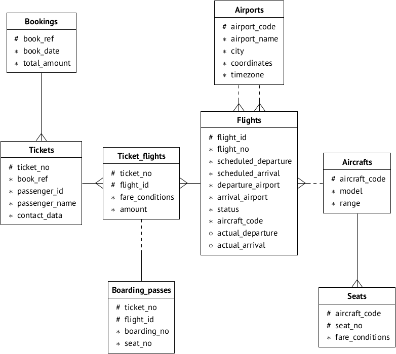
We will take the database as ready-made: air transportation demobase , which is used by Postgres Professional training materials. On this page, you can select the base variant to your taste (that is, by size) and read its description. We reproduce the data scheme for convenience: Suppose that the base is installed on the server 192.168.1.100 and is called . Connecting:
democon <- dbConnect(drv, dbname = "demo",
host = "192.168.1.100", port = 5434,
user = "u_r")We continue. Let's see here with such a request which cities are most often delayed flights:
SELECT ap.city, avg(extract(EPOCH FROM f.actual_arrival) - extract(EPOCH FROM f.scheduled_arrival))/60.0 t FROM airports ap, flights f WHERE ap.airport_code = f.departure_airport AND f.scheduled_arrival < f.actual_arrival AND f.departure_airport = ap.airport_code GROUPBY ap.city ORDERBY t DESCLIMIT10;To obtain minutes of lateness, we used the postgres construct
extract(EPOCH FROM ...)to extract the “absolute” seconds from the type field timestampand divided it into 60.0, rather than 60, to avoid discarding the remainder of the division, understood as an integer. EXTRACT MINUTEcan not be used, as there are more than an hour late. We average the lateness of the operator avg. We transfer the text to a variable and send a request to the server:
sql1 <- "SELECT ... ;"
res1 <- dbGetQuery(con, sql1)
Now we will understand in what form the request came. For this, R has a function
class()class (res1)It will show that the result was packed into a type
data.frame, that is, we recall, an analogue of the base table: in fact, it is a matrix with columns of arbitrary types. She, by the way, knows the names of the columns, and you can refer to the columns, if anything, for example, like this:print (res1$city)It's time to think about how to visualize the results. To do this, you can see what we have. For example, select the appropriate graphics from this list :
- R-Bar Charts (line)
- R-Boxplots (stock)
- R-Histograms (histograms)
- R-Line Graphs (graphics)
- R-Scatterplots (point)
It should be borne in mind that for each type of input a suitable data type is supplied for the image. Choose a bar chart (recumbent bars). It requires two vectors for axis values. The “vector” type in R is just a set of similar values.
c()- vector constructor. You can form the necessary two vectors from the type result like
data.framethis:Time <- res1[,c('t')]
City <- res1[,c('city')]
class (Time)
class (City)The expressions in the right parts look weird, but this is a convenient technique. Moreover, in R it is possible to write various expressions in a very compact manner. In square brackets before the comma, the index of the series, after the comma - the index of the column. The fact that there is nothing in front of a comma means that all values from the corresponding column will be selected.
The Time class is obtained
numeric, and the City class is character. These are varieties of vectors. Now you can do the most visualization. You need to set the image file.
png(file = "/home/igor_le/R/pics/bars_horiz.png")After this follows a nudity procedure: set the parameters (
par) of the graphs. And do not say that everything in the graphics packages R was intuitive. For example, the parameter lasdetermines the position of labels with values along the axes relative to the axes themselves:- 0 and by default - parallel to the axes;
- 1 is always horizontal;
- 2 - perpendicular to the axes;
- 3 - always upright
All parameters will not be painted. In general, there are many: fields, scales, colors - look for, experiment at your leisure.
par(las=1)
par(mai=c(1,2,1,1))
Finally, we build a graph of recumbent columns:
barplot(Time, names.arg=City, horiz=TRUE, xlab="Опоздание (мин)", col="green", main="Среднее время опоздания", border="red", cex.names=0.9)This is not all. Last but not least:
dev.off()
For a change, let's draw a scatter chart of tardiness. Remove LIMIT from the query, the rest is the same. But the scatterplot needs one vector, not two.
Dots <- res2[,c('t')]
png(file = "/home/igor_le/R/scripts/scatter.png")
plot(input5, xlab="Кучность",ylab="Опоздания",main="Распределение опозданий")
dev.off()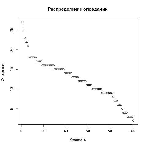
For visualization we used standard packages. It is clear that R is a popular language and packages exist at roughly infinity. You can ask about the already installed ones:
library()Part II. R generates retirees
R is convenient to use not only for data analysis, but also for their generation. Where there are rich statistical functions, there can not be a variety of algorithms for creating random sequences. In particular, you can use typical (Gaussian) and not quite typical (Zipf) distributions for simulating database requests.
But about it in the following part.