September 22, 2015 at 10:12
The spectral method as an example of simple problems of mathematics
This article describes the pseudo-spectral method for the numerical solution of the equations of mathematics used in computational fluid dynamics, geophysics, climatology and many other fields.
To begin with, we consider a simple one-dimensional heat distribution problem in a rod. An equation describing the distribution of heat at a certain initial temperature distribution over the rod:


This equation is solved analytically by the method of separation of variables, for example here , but we are interested in how this can be done numerically. First of all, you need to decide how to calculate the second spatial derivative with respect to x. This is most easily done by some difference method, for example:

But we will act differently. The temperature distribution is a function of the coordinate and time, and at each moment of time this function can be represented as the sum of the Fourier series, which is numerically cut off on the nth term:

Where u ^ "with a cap" are the expansion coefficients of the Fourier series. We substitute the expression for the series into the heat transfer equation:

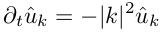
We obtain the equation for the Fourier coefficients, in which there is no derivative with respect to the coordinate! Now this is an ordinary differential equation, and not in partial derivatives, which can be solved by a simple difference method. Already easier, now it remains to find the expansion coefficients, and the Fourier transform (hereinafter referred to as FFT) will greatly help us .
The logic here is as follows:
1) at the initial moment of time, a coordinate function is given that describes the temperature distribution over the rod;
2) break the rod into a grid of n points;
3) we find the complex Fourier coefficients using the FFT algorithm, denote the operation as F (u);
4) we multiply the obtained coefficients by - | k | 2 , we obtain the Fourier transform of the second derivative. Similarly, you can get the Fourier transform of a derivative of higher orders p, just multiply by (ik) p ;
5) we do the inverse Fourier transform F -1 (u), using the IFFT algorithm, we obtain the values of the second derivative at points on the grid;
6) we take a time step, already the usual difference, explicit or implicit, scheme;
7) repeat.
Now let's see how it works in the program for Matlab / Octave. As the initial temperature distribution, we take the smooth function u0 = 2 + sin (x) + sin (2x), we divide a rod with a length of 2π into 50 points, with a time step of h = 0.1, the boundary conditions are periodic (ring).
It is worth noting a feature of the FFT algorithm in Matlab related to the fact that the obtained expansion coefficients at the output d = fft (u) are not in order, but are shifted, the first half is in place of the second and vice versa. First, there are coefficients with numbers from 0 to n / 2-1, then with numbers from -n / 2 to -1. There were problems with this ...

The solution obtained can be seen on the graph in the form of a “waterfall” of temperature distribution lines along x for each time t. It can be seen that the solution experiencesstrong oscillations of numerical instability, this is due to the failure of the Courant criterion . You can get rid of instability by decreasing the time step, or by applying a more advanced implicit scheme, for example, Crank-Nicholson .


Initial conditions: u0 = 1 + sin (2X) + cos (2Y), where u is now a 2d-array u (i, j). We use the implicit time integration scheme (i.e., we express the m + 1 step in terms of the mth):


We can prove that such an implicit scheme never diverges for η> 0.5, we use η = 1. Thus, each new value u m + 1 is obtained by multiplying u m by a coefficient μ k depending on the time step and wave numbers k, i.e. μ k is a constant that does not need to be counted at every step!


There is a second time derivative in the wave equation, therefore the task is reduced to a system of two ordinary diffurs, one variable is u, the second is u t , the time scheme in the code used the simplest explicit one, therefore the accuracy is small, the time step is very small, but the code It looks relatively simple. However, this is enough to demonstrate the operability of the method.
Periodic boundary conditions:
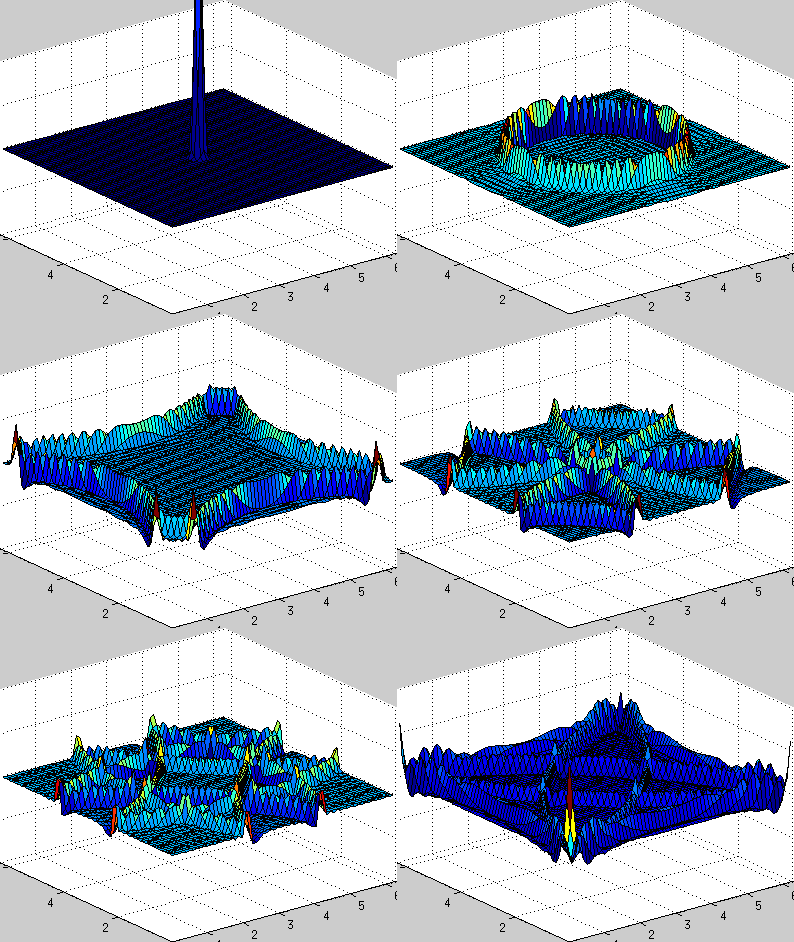
Fixed boundary conditions (0 at the edges, reflection of waves from the boundaries):
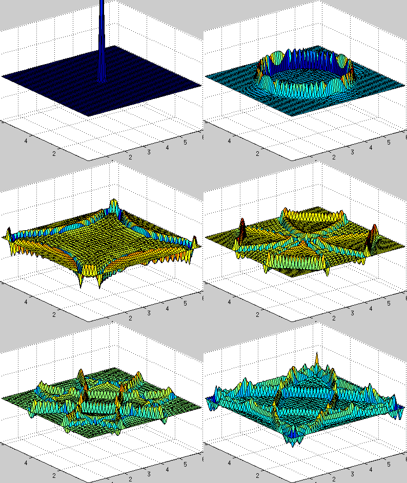
The article demonstrates several examples of the application of the spectral method for simple problems of mathematics. The main essence of the spectral method is the replacement of the original partial differential equations with ordinary diffurs for the coefficients of the expansion of the desired functions in some basis. The basis can be sine cosines, complex exponentials, orthogonal polynomials, if geometry requires - cylindrical or spherical functions. The found coefficients at each moment of time allow you to restore the desired solution, and the FFT algorithm allows you to do this quickly.
The advantages of the method are:
Disadvantages are also available:
I hope my first article will be useful to someone, at least this is a possible start for those who study this section of numerical methods. Waiting for critical comments on the code , design and tips!
The one-dimensional problem of heat propagation along the rod
To begin with, we consider a simple one-dimensional heat distribution problem in a rod. An equation describing the distribution of heat at a certain initial temperature distribution over the rod:
This equation is solved analytically by the method of separation of variables, for example here , but we are interested in how this can be done numerically. First of all, you need to decide how to calculate the second spatial derivative with respect to x. This is most easily done by some difference method, for example:
But we will act differently. The temperature distribution is a function of the coordinate and time, and at each moment of time this function can be represented as the sum of the Fourier series, which is numerically cut off on the nth term:
Where u ^ "with a cap" are the expansion coefficients of the Fourier series. We substitute the expression for the series into the heat transfer equation:
We obtain the equation for the Fourier coefficients, in which there is no derivative with respect to the coordinate! Now this is an ordinary differential equation, and not in partial derivatives, which can be solved by a simple difference method. Already easier, now it remains to find the expansion coefficients, and the Fourier transform (hereinafter referred to as FFT) will greatly help us .
The logic here is as follows:
1) at the initial moment of time, a coordinate function is given that describes the temperature distribution over the rod;
2) break the rod into a grid of n points;
3) we find the complex Fourier coefficients using the FFT algorithm, denote the operation as F (u);
4) we multiply the obtained coefficients by - | k | 2 , we obtain the Fourier transform of the second derivative. Similarly, you can get the Fourier transform of a derivative of higher orders p, just multiply by (ik) p ;
5) we do the inverse Fourier transform F -1 (u), using the IFFT algorithm, we obtain the values of the second derivative at points on the grid;
6) we take a time step, already the usual difference, explicit or implicit, scheme;
7) repeat.
Now let's see how it works in the program for Matlab / Octave. As the initial temperature distribution, we take the smooth function u0 = 2 + sin (x) + sin (2x), we divide a rod with a length of 2π into 50 points, with a time step of h = 0.1, the boundary conditions are periodic (ring).
Code for the one-dimensional heat transfer equation
clear all;
n = 50;             % number of points
dx = 2*pi/n;        % space step
x = 0:dx:2*pi-dx;   % grid
h = 0.1;            % temporal step
times = 10;         % number of iterations in time
k = fftshift(-n/2:1:n/2-1); % wave numbers
k2 = k.*k;
u0 = 2 + sin(x) + sin(2*x); % initial conditions
u = zeros(times,n);         % stores results
u(1,:) = u0;
uf = fft(u0);                  % Fourier coefficients of initial function
for i=2:times
    uf = uf.*(1-h*k2);      % next time step in Fourier space
    u(i,:) = real(ifft(uf));  % IFFT to physical space
end
[X,T] = meshgrid(x,0:h:times*h-h);
waterfall(X,T,u)
It is worth noting a feature of the FFT algorithm in Matlab related to the fact that the obtained expansion coefficients at the output d = fft (u) are not in order, but are shifted, the first half is in place of the second and vice versa. First, there are coefficients with numbers from 0 to n / 2-1, then with numbers from -n / 2 to -1. There were problems with this ...
The solution obtained can be seen on the graph in the form of a “waterfall” of temperature distribution lines along x for each time t. It can be seen that the solution experiences
Two-dimensional diffusion equation
Initial conditions: u0 = 1 + sin (2X) + cos (2Y), where u is now a 2d-array u (i, j). We use the implicit time integration scheme (i.e., we express the m + 1 step in terms of the mth):
We can prove that such an implicit scheme never diverges for η> 0.5, we use η = 1. Thus, each new value u m + 1 is obtained by multiplying u m by a coefficient μ k depending on the time step and wave numbers k, i.e. μ k is a constant that does not need to be counted at every step!
Code for the two-dimensional diffusion equation
clear all;
eta = 1;
n = 32;              % number of points
dx = 2*pi/n;         % space step
x = 0:dx:2*pi-dx;
y = x;
[X, Y] = meshgrid(x,y);
h = 0.01;            % temporal step
times = 30;         % number of iterations in time
k1 = meshgrid(fftshift(-n/2:1:n/2-1),ones(n,1));
k2 = k1';
ks = k1.*k1 + k2.*k2;
mu = (1-(1-eta)*ks^2*h)./(1+eta*ks.^2*h); % stores multipliers
u0 = 1 + sin(2*X) + sin(2*Y);  % initial temperature
u = zeros(times,n,n);        % stores results
umin=min(min(u0));
umax=max(max(u0));
u(1,:,:) = u0;
uf = fft2(u0);
for i=2:times
    uf = mu.*uf;  % time step
    u(i,:,:) = real(ifft2(uf));
end
createGif('diffusion2d.gif',X,Y,u,times,1,[0 2*pi 0 2*pi umin umax]);
Saving GIFs
function createGif(name,X,Y,u,times,every,ax)
% creates gif movie form 3D array
% save results to gif file
gifka = name;
clf;
pic = surf(X,Y,squeeze(u(1,:,:))),axis(ax);
for i=1:every:times
    set(pic,'zdata',squeeze(u(i,:,:))), drawnow;
    M(i) = getframe;
    frame = getframe;
    im = frame2im(frame);
    [imind,cm] = rgb2ind(im,256);
    if i == 1;
        imwrite(imind,cm,gifka,'gif','Loopcount',inf);
    else
        imwrite(imind,cm,gifka,'gif','WriteMode','append','DelayTime',.1);
    end
end
end
Two-dimensional wave equation
There is a second time derivative in the wave equation, therefore the task is reduced to a system of two ordinary diffurs, one variable is u, the second is u t , the time scheme in the code used the simplest explicit one, therefore the accuracy is small, the time step is very small, but the code It looks relatively simple. However, this is enough to demonstrate the operability of the method.
Code for two-dimensional wave equation
clear all;
a = 1;               % speed of wave propagation
n = 64;              % number of points
dx = 2*pi/n;         % space step
x = 0:dx:2*pi-dx;
y = x;
[X, Y] = meshgrid(x,y);
h = 0.01;            % temporal step
times = 1000;         % number of iterations in time
% explanation of this part is here www.staff.uni-oldenburg.de/hannes.uecker/pre/030-mcs-hu.pdf
k1 = meshgrid(fftshift(-n/2:1:n/2-1),ones(n,1));
k2 = k1';
ks = k1.*k1 + k2.*k2;
u0 = exp(-100*((X-pi).^2 + (Y-pi).^2));  % profile of initial velocity u
ut0 = zeros(n,n);                           % profile of initial acceleration ut
u = zeros(times,n,n);  % stores velocity profile for every time steps
u(1,:,:) = u0;
uf = fft2(u0);
uft = fft2(ut0);
for i=2:times
    uft_new = uft - a*h*ks.*uf;
    uf = uf + 0.5*h*(uft+uft_new);
    uft = uft_new;
    % == fixed boundary conditions
%     u0 = real(ifft2(uf));
%     u0(1,:) = 0; u0(end,:) = 0;
%     u0(:,1) = 0; u0(:,end) = 0;
%     uf = fft2(u0);
    % == fixed boundary conditions
    u(i,:,:) = real(ifft2(uf));
end
createGif('wave2d_periodic_bc.gif',X,Y,u,times,10,[0 2*pi 0 2*pi -.2 .2]);
Periodic boundary conditions:
Fixed boundary conditions (0 at the edges, reflection of waves from the boundaries):
conclusions
The article demonstrates several examples of the application of the spectral method for simple problems of mathematics. The main essence of the spectral method is the replacement of the original partial differential equations with ordinary diffurs for the coefficients of the expansion of the desired functions in some basis. The basis can be sine cosines, complex exponentials, orthogonal polynomials, if geometry requires - cylindrical or spherical functions. The found coefficients at each moment of time allow you to restore the desired solution, and the FFT algorithm allows you to do this quickly.
The advantages of the method are:
- Good accuracy for "good" features. As the number of grid points n increases, the error of the finite difference method decreases as O (N -m )) (where m is a certain constant that depends on the order of the method and the smoothness of the function), and for the spectral method, the accuracy can be exponential O (c N ), where 0 <c <1.
- The relative ease of use, especially when finding derivatives of high degrees, for comparison, the finite difference method involves the use of rather complex formulas. The use of the effective FFT algorithm gives O (N log (N)) complexity, which is acceptable for large enough problems
- The spectral method is effective with respect to memory; therefore, it is widely used in geophysics, climate modeling, and meteorology.
Disadvantages are also available:
- Gibbs phenomenon , a very bad phenomenon, strongly affecting the accuracy at the edges of the region
- More demanding on computing resources for a degree of freedom than in difference methods
- It is poorly applicable to problems with non-standard geometry, and boundary conditions other than periodic.
I hope my first article will be useful to someone, at least this is a possible start for those who study this section of numerical methods. Waiting for critical comments on the code , design and tips!
Sources used
- Great review from Hannes Uecker with code examples , some of which I used in this article
- A small and therefore wonderful book by Lloyd N. Trefethen, Spectral Methods in MATLAB
- Fundamental book by John P. Boyd “Chebyshev and Fourier Spectral Methods”