Preparing t-SNE
- Tutorial
While working on the article “Deep Learning on R ...” , I several times mentioned the mention of t-SNE - the mysterious technique of nonlinear dimensionality reduction and visualization of multidimensional variables (for example, here ), I was intrigued and decided to figure out everything in detail. t-SNE is a t-distributed stochastic neighbor embedding . The Russian version with the “introduction of neighbors” sounds ridiculous to some extent, so I will continue to use the English acronym.
The t-SNE algorithm, which is also referred to as multiple feature training methods, was published in 2008 (ref. 1 at the end of the article) by Dutch researcher Lawrence van der Maaten (now works at Facebook AI Research) and neural network sorcerer Jeffrey Hinton. The classic SNE was proposed by Hinton and Roways in 2002 (Ref. 2). The 2008 article described several “tricks” that made it possible to simplify the process of searching for global lows and improve the quality of visualization. One of them was the replacement of the normal distribution by the Student distribution for low-dimensional data. In addition, a successful implementation of the algorithm was made (the article has a link to MatLab), which was then ported to other popular environments .
Let's start with the “classic” SNE and formulate the problem. We have a data set with points described by a multidimensional variable with a space dimension substantially greater than three. It is necessary to obtain a new variable that exists in two-dimensional or three-dimensional space, which would to the maximum extent preserve the structure and patterns in the source data. SNE begins by transforming the multidimensional Euclidean distance between points into conditional probabilities that reflect the similarity of points. Mathematically, it looks like this (formula 1):

This formula shows how close the point X j is to the point X i with a Gaussian distribution around X iwith a given deviation σ. Sigma will be different for each point. It is chosen so that points in areas with a higher density have less dispersion. For this, the perplexity estimate is used :

Where H (Pi) is the Shannon entropy in bits (formula 2):

In this case, perplexity can be interpreted as a smoothed estimate of the effective number of "neighbors" for the point X i . It is set as a parameter to the method. The authors recommend using a value between 5 and 50. Sigma is determined for each pair X i and X j using a binary search algorithm .
For two-dimensional or three-dimensional "colleagues" pairs X i and X j, let's call them Y i and Y j for clarity , it is not difficult to estimate the conditional probability using the same formula 1. The standard deviation is proposed to be set to 1 / √2:

If the display points Y i and Y j correctly model the similarity between the source points of high dimension X i and X j , then the corresponding conditional probabilities p j | i and q j | i will be equivalent. As an obvious estimate of the quality with which q j | i reflects p j | i , the divergence or Kullback-Leibler distance is used. SNE minimizes the sum of such distances for all display points using gradient descent. The loss function for this method will be determined by formula 3:

In this case, the gradient looks surprisingly simple:

The authors offer the following physical analogy for the optimization process: All display points are connected by springs. The stiffness of the spring connecting the points i and j depends on the difference between the similarities of two points in multidimensional space and two points in the display space. In this analogy, a gradient is the resulting force acting on a point in the display space. If you let the system go, after a while it will come to equilibrium, this will be the desired distribution. Algorithmically, the search for equilibrium is proposed to be done taking into account the moments:

where η is a parameter that determines the learning speed (step length), and α is the inertia coefficient. Using the classic SNE allows you to get good results, but it can be connected with difficulties in optimizing the loss function and the crowding problem (in the original - crowding problem). t-SNE even if it does not solve these problems at all, it greatly facilitates. The loss function of t-SNE has two fundamental differences. Firstly, t-SNE has a symmetric form of similarity in multidimensional space and a simpler version of the gradient. Secondly, instead of a Gaussian distribution for points from the display space, a t-distribution (Student's) is used, whose “heavy” tails facilitate optimization and solve the crowding problem.
As an alternative to minimizing the sum of Kullback-Leibler divergences between conditional probabilities pi | j and q i | j, it is proposed to minimize the single divergence between the joint probability P in multidimensional space and the joint probability Q in the mapping space:

where p ii and q ii = 0, p ij = p ji , q ij = q ji for any i and j, and p ij is determined by the formula:

where n is the number of points in the data set. The gradient for symmetric SNE is much simpler than for the classical one:

The problem of crowding is that the distance between two points in the display space corresponding to two mid-distance points in a multidimensional space should be significantly larger than the distance that allows you to get a Gaussian distribution. Student tails solve the problem. The t-SNE uses a t-distribution with one degree of freedom. The joint probability for the display space in this case will be determined by the formula 4:
And the corresponding gradient by the expression 5:

Returning to the physical analogy, the resulting force defined by formula 5 will significantly contract the points of the display space for nearby points of the multidimensional space, and repel them for the remote .
The t-SNE algorithm in a simplified form can be represented by the following pseudo-code:
To improve the result, it is proposed to use two tricks. The first authors called "early compression". Its task is to make the points in the display space at the beginning of optimization be as close to each other as possible. When the distance between the display points is small, moving one cluster through another is much easier. It’s much easier to explore the optimization space and “target” global lows. Early compression is created due to an additional L2 penalty in the loss function, which is proportional to the sum of the squares of the distances of the display points from the origin (I did not find this in the source code).
The second trick is less obvious - "early hyper-amplification" (in the original - "early exaggeration"). It consists in multiplying at the beginning of the optimization of all p ijfor some integer, such as 4. The point is that for large p ij get make greater q ij . This will allow for clusters in the source data to obtain dense and widely spaced clusters in the display space.
As the source code, I took the original MatLab implementation of van der Maaten. However, the academic license for MatLab has long expired, so I ported all the code to R. The code is available in the repository . Also, I had at my disposal a code from the archive of the tsne R-package , took a couple of ideas from there.
For experiments it is proposed to use the following parameters:
Number of iterations: 1000;
Perplexia: 40;
Early hyperpower: x4 for the first 50 iterations;
Moment α: 0.5 for the first 250 iterations, 0.8 for the remaining 750;
Learning speed η: initially 100 (in the original code - 500) and changes after each iteration in accordance with the scheme described by Robert Jacobs in 1988 (ref. 3).
The algorithm can be divided into three logical parts:
I will illustrate only the most important designs. First of all, it is necessary to calculate the square matrix of the Euclidean distance for the original data set. To do this, it is better to use the rdist () function from the fields package. It works many times faster than the popular dist () from the basic stats package. Perhaps this is because it is optimized specifically for the Euclidean distance. Next, you need to initialize the display space. This can be done using rnorm () with a zero mat. expectation and standard deviation 1e-4.
The calculation of the logarithm of perplexity and the Gaussian core is as follows:
The last expression is obtained if formula (1) for p j | i is substituted by formula (2) for perplexity. Let n be the number of points in the source data. Di is a vector of length n-1, with squares of pairwise distances for the line of the source data. It is obtained using the construction Di <- D [i, -i] , where D is the matrix of squares of distances nxn, and if i = 1, then Di is the first row of the matrix D without the first column. The kernel, P is a vector of length n-1, and the logarithm of perplexia is a real number (due to the sum before the element-wise product). The original code uses the natural logarithm, I decided to do the same.
For gamma search there are the following restrictions - the number of attempts (divisions) is not more than 50, the threshold for the difference between the logarithms of the given and calculated perplexity is 1e-5. One iteration of a binary search is as follows:
gammamin and gammamax are initially installed in - and + Inf .
The loss function is considered as the sum over the rows of the element-wise product of two nxn matrices:
P is the symmetric version of the joint probability for a multidimensional space; it is calculated as P = .5 * (P + t (P)) from the conditional pairwise probability, t is the matrix transpose operator. Q is the joint probability for the display space:
Y is the initialized matrix of points nx 2 for the two-dimensional display space. Q is obtained by nxn by using rdist () .
The gradient is calculated in a vectorized form at once for all Yi:
Here grads is an nx 2 matrix that is formed by the matrix product. The construction in parentheses is a matrix of size nxn, on the main diagonal of which line-by-line sums of matrix L, and all other elements are taken with a minus sign. The matrix product allows you to multiply by the difference Y i and Y j and immediately calculate the sum by j (formula 4). True gradient is obtained by the opposite sign.
To search for optimal values of Y, something similar to the delta-bar-delta Robert Jacobs heuristic is used. Its meaning is to adaptively change the learning step. If the gradient does not change its sign at the next iteration, the step increases linearly (0.2 is added to the gain), if the sign changes, it decreases exponentially (the coefficient is multiplied by 0.8). Given that the gradient we have is the opposite sign:
I could not help but try to repeat the experiment described in the article (link 1). The idea of this experiment is to visualize the cluster structure for the MNIST image set. One part of this set contains 60,000 images of handwritten numbers from 0 to 9, 28x28 pixels. The dataset can be downloaded from the site of the neuron network guru, Jan Lekun.
You will have to tinker with loading into R, but the readBin () function helps, which allows you to read (and write) binary data. 20 random digits:

As in the original experiment, I did not use the entire set, but only 6,000 images randomly selected using the sample () function . 1000 iterations took a little less than an hour and a half on x64 with Intel Core i7 2.4 GHz. The result in the picture:

Colors are set using labels, MNIST is a labeled dataset. The result can be significantly improved. As the authors advise, for the initial set of points, you should do a principal component analysis (PCA) and select the first 30:

There are several PCA implementations for R. The simplest option is in two lines:
The speed of the algorithm is proportional to the square of the number of points. If this amount is reduced, the result will not be so obvious, but quite acceptable. Say 2000 points are processed in just 9 minutes.
The t-SNE technique would probably not be so popular if not for the ability to visualize a distributed representation of words. In this experiment, I used a relatively small model (about 900 words and a 300-dimensional attribute space), trained with word2vec .

Here the size is bigger. A three-dimensional display space is used, the third dimension is represented by color. Words can be considered close if they are located nearby and have the same connotation.
It turns out that with a distributed representation of words prepared on real data, it is not so simple. There are two problems: as a rule, a very large number of clusters and significant differences in their size. For visualization, you can make a random selection, but the result will most likely not be representative. The authors explain this with the following example: If A, B, and C are equidistant points in a multidimensional space, but there are still points between A and B and there are no points between B and C, then the algorithm is more likely to combine A and B into one cluster than B and C.
But it sometimes happens that the clarity is important, not the completeness of the picture. Then, instead of randomly selecting points, you can try to select interesting clusters. Clustering is built into the original word2vec, in addition, you can use k-means. Perhaps this option does not seem completely “honest”, but, in my opinion, it has the right to exist. Fetching data for a distributed representation of words from fifteen clusters doesn’t seem so confusing anymore:
For large data sets, there is a special t-SNE implementation in which nearest neighbor trees and a random walk method are used to calculate similarities in multidimensional space (described in article 1). In practice, you can use the Rtsne package, a wrapper for the C ++ implementation of Barnes-Hut-SNE. Rtsne can process all 60,000 MNIST images in less than an hour. Details can be found in publication 6.
I have not experimented with Rtsne yet, but I have tested tsne (the port of the MatLab code for R). Visualization is much worse than my version. Looking at the package archive, I found two things: Firstly, when calculating the Gaussian core, the distance is used without squared, and secondly, the matrix product is in the expression for perplexity. In my version and in the code for MatLab, it is element-wise. It is strange that generally visible clusters were obtained. I explain this by the “survivability” of the algorithm, but I admit that I did not fully understand something. I will be glad to comments and I wish you all an impressive multi-dimensional visualization.
The formulas for this article have been prepared using the LATEX online formula editor .
The t-SNE algorithm, which is also referred to as multiple feature training methods, was published in 2008 (ref. 1 at the end of the article) by Dutch researcher Lawrence van der Maaten (now works at Facebook AI Research) and neural network sorcerer Jeffrey Hinton. The classic SNE was proposed by Hinton and Roways in 2002 (Ref. 2). The 2008 article described several “tricks” that made it possible to simplify the process of searching for global lows and improve the quality of visualization. One of them was the replacement of the normal distribution by the Student distribution for low-dimensional data. In addition, a successful implementation of the algorithm was made (the article has a link to MatLab), which was then ported to other popular environments .
A bit of math
Let's start with the “classic” SNE and formulate the problem. We have a data set with points described by a multidimensional variable with a space dimension substantially greater than three. It is necessary to obtain a new variable that exists in two-dimensional or three-dimensional space, which would to the maximum extent preserve the structure and patterns in the source data. SNE begins by transforming the multidimensional Euclidean distance between points into conditional probabilities that reflect the similarity of points. Mathematically, it looks like this (formula 1):
This formula shows how close the point X j is to the point X i with a Gaussian distribution around X iwith a given deviation σ. Sigma will be different for each point. It is chosen so that points in areas with a higher density have less dispersion. For this, the perplexity estimate is used :
Where H (Pi) is the Shannon entropy in bits (formula 2):
In this case, perplexity can be interpreted as a smoothed estimate of the effective number of "neighbors" for the point X i . It is set as a parameter to the method. The authors recommend using a value between 5 and 50. Sigma is determined for each pair X i and X j using a binary search algorithm .
For two-dimensional or three-dimensional "colleagues" pairs X i and X j, let's call them Y i and Y j for clarity , it is not difficult to estimate the conditional probability using the same formula 1. The standard deviation is proposed to be set to 1 / √2:
If the display points Y i and Y j correctly model the similarity between the source points of high dimension X i and X j , then the corresponding conditional probabilities p j | i and q j | i will be equivalent. As an obvious estimate of the quality with which q j | i reflects p j | i , the divergence or Kullback-Leibler distance is used. SNE minimizes the sum of such distances for all display points using gradient descent. The loss function for this method will be determined by formula 3:
In this case, the gradient looks surprisingly simple:
The authors offer the following physical analogy for the optimization process: All display points are connected by springs. The stiffness of the spring connecting the points i and j depends on the difference between the similarities of two points in multidimensional space and two points in the display space. In this analogy, a gradient is the resulting force acting on a point in the display space. If you let the system go, after a while it will come to equilibrium, this will be the desired distribution. Algorithmically, the search for equilibrium is proposed to be done taking into account the moments:
where η is a parameter that determines the learning speed (step length), and α is the inertia coefficient. Using the classic SNE allows you to get good results, but it can be connected with difficulties in optimizing the loss function and the crowding problem (in the original - crowding problem). t-SNE even if it does not solve these problems at all, it greatly facilitates. The loss function of t-SNE has two fundamental differences. Firstly, t-SNE has a symmetric form of similarity in multidimensional space and a simpler version of the gradient. Secondly, instead of a Gaussian distribution for points from the display space, a t-distribution (Student's) is used, whose “heavy” tails facilitate optimization and solve the crowding problem.
As an alternative to minimizing the sum of Kullback-Leibler divergences between conditional probabilities pi | j and q i | j, it is proposed to minimize the single divergence between the joint probability P in multidimensional space and the joint probability Q in the mapping space:
where p ii and q ii = 0, p ij = p ji , q ij = q ji for any i and j, and p ij is determined by the formula:
where n is the number of points in the data set. The gradient for symmetric SNE is much simpler than for the classical one:
The problem of crowding is that the distance between two points in the display space corresponding to two mid-distance points in a multidimensional space should be significantly larger than the distance that allows you to get a Gaussian distribution. Student tails solve the problem. The t-SNE uses a t-distribution with one degree of freedom. The joint probability for the display space in this case will be determined by the formula 4:
And the corresponding gradient by the expression 5:
Returning to the physical analogy, the resulting force defined by formula 5 will significantly contract the points of the display space for nearby points of the multidimensional space, and repel them for the remote .
Algorithm
The t-SNE algorithm in a simplified form can be represented by the following pseudo-code:
Data: data set X = {x1, x2, ..., xn},
loss function parameter: Perp perplexia,
Optimization parameters: number of iterations T, learning rate η, moment α (t).
Result: data representation Y (T) = {y1, y2, ..., yn} (in 2D or 3D).
begin
	calculate pairwise similarity pj | ic with Perp perplexia (using formula 1)
	set pij = (pj | i + pi | j) / 2n
	initialize Y (0) = {y1, y2, ..., yn} with points of normal distribution (mean = 0, sd = 1e-4)
	for t = 1 to T do
 		calculate the similarity of points in the mapping space qij (by formula 4)
		calculate the gradient δCost / δy (according to formula 5)
		set Y (t) = Y (t-1) + ηδCost / δy + α (t) (Y (t-1) - Y (t-2))
	end
end
To improve the result, it is proposed to use two tricks. The first authors called "early compression". Its task is to make the points in the display space at the beginning of optimization be as close to each other as possible. When the distance between the display points is small, moving one cluster through another is much easier. It’s much easier to explore the optimization space and “target” global lows. Early compression is created due to an additional L2 penalty in the loss function, which is proportional to the sum of the squares of the distances of the display points from the origin (I did not find this in the source code).
The second trick is less obvious - "early hyper-amplification" (in the original - "early exaggeration"). It consists in multiplying at the beginning of the optimization of all p ijfor some integer, such as 4. The point is that for large p ij get make greater q ij . This will allow for clusters in the source data to obtain dense and widely spaced clusters in the display space.
Implementation on R
As the source code, I took the original MatLab implementation of van der Maaten. However, the academic license for MatLab has long expired, so I ported all the code to R. The code is available in the repository . Also, I had at my disposal a code from the archive of the tsne R-package , took a couple of ideas from there.
For experiments it is proposed to use the following parameters:
Number of iterations: 1000;
Perplexia: 40;
Early hyperpower: x4 for the first 50 iterations;
Moment α: 0.5 for the first 250 iterations, 0.8 for the remaining 750;
Learning speed η: initially 100 (in the original code - 500) and changes after each iteration in accordance with the scheme described by Robert Jacobs in 1988 (ref. 3).
The algorithm can be divided into three logical parts:
- Calculation of perplexity and the Gaussian kernel for the vector of current sigma values (or rather gamma, I used the inverse of the sigma square)
- Calculation of pairwise similarity p ij in multidimensional space using binary search for a given perplexity
- Calculation of pairwise similarities for display space, loss function and gradient
I will illustrate only the most important designs. First of all, it is necessary to calculate the square matrix of the Euclidean distance for the original data set. To do this, it is better to use the rdist () function from the fields package. It works many times faster than the popular dist () from the basic stats package. Perhaps this is because it is optimized specifically for the Euclidean distance. Next, you need to initialize the display space. This can be done using rnorm () with a zero mat. expectation and standard deviation 1e-4.
The calculation of the logarithm of perplexity and the Gaussian core is as follows:
P <- exp(-Di * gamma) # kernel calc
sumP <- sum(P)
PP <- log(sumP) + gamma * sum(Di * P) / sumP
The last expression is obtained if formula (1) for p j | i is substituted by formula (2) for perplexity. Let n be the number of points in the source data. Di is a vector of length n-1, with squares of pairwise distances for the line of the source data. It is obtained using the construction Di <- D [i, -i] , where D is the matrix of squares of distances nxn, and if i = 1, then Di is the first row of the matrix D without the first column. The kernel, P is a vector of length n-1, and the logarithm of perplexia is a real number (due to the sum before the element-wise product). The original code uses the natural logarithm, I decided to do the same.
For gamma search there are the following restrictions - the number of attempts (divisions) is not more than 50, the threshold for the difference between the logarithms of the given and calculated perplexity is 1e-5. One iteration of a binary search is as follows:
            if (perpDiff > 0){
                   gammamin = gamma[i]
                   if (is.infinite(gammamax)) gamma[i] = gamma[i] * 2
                   else gamma[i] = (gamma[i] + gammamax)/2
            } else{
                   gammamax = gamma[i]
                   if (is.infinite(gammamin))  gamma[i] = gamma[i]/ 2
                   else gamma[i] = ( gamma[i] + gammamin) / 2
            }
gammamin and gammamax are initially installed in - and + Inf .
The loss function is considered as the sum over the rows of the element-wise product of two nxn matrices:
cost = sum(apply(P * log(P/Q),1,sum))
P is the symmetric version of the joint probability for a multidimensional space; it is calculated as P = .5 * (P + t (P)) from the conditional pairwise probability, t is the matrix transpose operator. Q is the joint probability for the display space:
            num = 1/(1 + (rdist(Y))^2)
            diag(num)=0 # Set diagonal to zero
            Q = num / sum(num) # Normalize to get probabilities
Y is the initialized matrix of points nx 2 for the two-dimensional display space. Q is obtained by nxn by using rdist () .
The gradient is calculated in a vectorized form at once for all Yi:
L = (P - Q) * num;
grads = 4 * (diag(apply(L, 1, sum)) - L) %*% Y
Here grads is an nx 2 matrix that is formed by the matrix product. The construction in parentheses is a matrix of size nxn, on the main diagonal of which line-by-line sums of matrix L, and all other elements are taken with a minus sign. The matrix product allows you to multiply by the difference Y i and Y j and immediately calculate the sum by j (formula 4). True gradient is obtained by the opposite sign.
To search for optimal values of Y, something similar to the delta-bar-delta Robert Jacobs heuristic is used. Its meaning is to adaptively change the learning step. If the gradient does not change its sign at the next iteration, the step increases linearly (0.2 is added to the gain), if the sign changes, it decreases exponentially (the coefficient is multiplied by 0.8). Given that the gradient we have is the opposite sign:
gains = (gains + .2) * abs(sign(grads) != sign(incs))
     + gains * .8 * abs(sign(grads) == sign(incs))
gains[gains < min_gain] = min_gain
incs = momentum * incs - gains  * epsilon * grads
 Y = Y + incs
The experiments
I could not help but try to repeat the experiment described in the article (link 1). The idea of this experiment is to visualize the cluster structure for the MNIST image set. One part of this set contains 60,000 images of handwritten numbers from 0 to 9, 28x28 pixels. The dataset can be downloaded from the site of the neuron network guru, Jan Lekun.
You will have to tinker with loading into R, but the readBin () function helps, which allows you to read (and write) binary data. 20 random digits:
As in the original experiment, I did not use the entire set, but only 6,000 images randomly selected using the sample () function . 1000 iterations took a little less than an hour and a half on x64 with Intel Core i7 2.4 GHz. The result in the picture:
Colors are set using labels, MNIST is a labeled dataset. The result can be significantly improved. As the authors advise, for the initial set of points, you should do a principal component analysis (PCA) and select the first 30:
There are several PCA implementations for R. The simplest option is in two lines:
pca <- prcomp(X)
X <- pca$x[,1:30]
The speed of the algorithm is proportional to the square of the number of points. If this amount is reduced, the result will not be so obvious, but quite acceptable. Say 2000 points are processed in just 9 minutes.
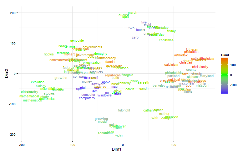
The t-SNE technique would probably not be so popular if not for the ability to visualize a distributed representation of words. In this experiment, I used a relatively small model (about 900 words and a 300-dimensional attribute space), trained with word2vec .
Here the size is bigger. A three-dimensional display space is used, the third dimension is represented by color. Words can be considered close if they are located nearby and have the same connotation.
It turns out that with a distributed representation of words prepared on real data, it is not so simple. There are two problems: as a rule, a very large number of clusters and significant differences in their size. For visualization, you can make a random selection, but the result will most likely not be representative. The authors explain this with the following example: If A, B, and C are equidistant points in a multidimensional space, but there are still points between A and B and there are no points between B and C, then the algorithm is more likely to combine A and B into one cluster than B and C.
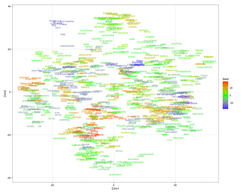
But it sometimes happens that the clarity is important, not the completeness of the picture. Then, instead of randomly selecting points, you can try to select interesting clusters. Clustering is built into the original word2vec, in addition, you can use k-means. Perhaps this option does not seem completely “honest”, but, in my opinion, it has the right to exist. Fetching data for a distributed representation of words from fifteen clusters doesn’t seem so confusing anymore:
For large data sets, there is a special t-SNE implementation in which nearest neighbor trees and a random walk method are used to calculate similarities in multidimensional space (described in article 1). In practice, you can use the Rtsne package, a wrapper for the C ++ implementation of Barnes-Hut-SNE. Rtsne can process all 60,000 MNIST images in less than an hour. Details can be found in publication 6.
I have not experimented with Rtsne yet, but I have tested tsne (the port of the MatLab code for R). Visualization is much worse than my version. Looking at the package archive, I found two things: Firstly, when calculating the Gaussian core, the distance is used without squared, and secondly, the matrix product is in the expression for perplexity. In my version and in the code for MatLab, it is element-wise. It is strange that generally visible clusters were obtained. I explain this by the “survivability” of the algorithm, but I admit that I did not fully understand something. I will be glad to comments and I wish you all an impressive multi-dimensional visualization.
The formulas for this article have been prepared using the LATEX online formula editor .
References:
- LJP van der Maaten and GE Hinton. Visualizing High-Dimensional Data Using t-SNE. Journal of Machine Learning Research 9 (Nov): 2579-2605, 2008. PDF
- GE Hinton and ST Roweis. Stochastic Neighbor Embedding. In Advances in Neural Information. Processing Systems, volume 15, pages 833–840, Cambridge, MA, USA, 2002. The MIT Press. Pdf
- RA Jacobs. Increased rates of convergence through learning rate adaptation. Neural Networks, 1: 295–307, 1988. PDF
- Python t-SNE Experiments: t-SNE Algorithm. Illustrated introductory course (translation of the original article on O'Reilly ). datareview.info/article/algoritm-t-sne-illyustrirovannyiy-vvodnyiy-kurs
- Rtsne vs. tsne: www.codeproject.com/Tips/788739/Visualization-of-High-Dimensional-Data-using-t-SNE A dataset is also available for experiments with a distributed representation of words.
- LJP van der Maaten. Accelerating t-SNE using Tree-Based Algorithms. Journal of Machine Learning Research 15 (Oct): 3221-3245, 2014. PDF