Tile Walk

For motorists, the problem of unfamiliar streets has long been solved by navigators. But even motorists walk. If the store is across the road, then we get up and go. Difficulties arise if you have to walk five hundred meters along an unfamiliar street and turn two or three times.

None of the services known to us built a route from point A to point B where there are no paths and sidewalks, but it is full of fences and houses of bizarre outlines.

2GIS solved this problem. We learned how to build routes for pedestrians on a rasterized map of the area. The map is formally represented by a graph with vertices on a regular grid in places where a pedestrian can be physically located.

It is generally accepted that such a way to build routes is unacceptable, because it eats up a lot of resources. Under the cut - how we dealt with it.

Algorithm

We will depict an algorithm for constructing a walking route.

1. We rasterize the area with a resolution of 2 × 2 meters. Rasterization includes houses, roads, fences, reservoirs, passages, ravines ... In the simplest case, each pixel gets a value - it is possible or impossible to go through. But nothing prevents the graduation of patency:
   
   • can go fast
   • you can go
   • difficult
   • don't get through
   Priority is important. We put obstacles on the initially passable terrain: houses, impassable roads, fences, ravines, railways ... Then we cut passable roads and pedestrian crossings with railway crossings in the form of circles with a diameter slightly wider than the road.
2. We consider the map of the area as a description of the graph with implicitly indicated relationships between neighboring cells. Transition only to passable, in which we have not been.
3. We work with the graph. If we are looking for a passage from point to point, we use a variant of algorithm A * .
   If we are looking for the nearest road, determining the passage to the nearest of the registered objects, then we start the search wave with the honest Dijkstra algorithm .
   

Two things scare in this pattern: memory and memory. Operational and on disk. Both that and that are spent too quickly. Let's try to solve the problem.

Fight for RAM

Each point has a potential of 8 pairs of edges - forward and backward. For a square kilometer it turns out: 500 × 500 × 8 = 2,000,000. If you act “on the forehead”, you have to process and save each ...

To save RAM, we divide the map into tiles of 256 × 256 cells or 512 × 512 meters. We will store only the perimeter of the wave, passing along the boundaries of the tiles. To store the perimeter, we’ll have a common “ heap ”.

Tiles are processed atomically. When pouring a tile, use its local “heap”. The algorithm is as follows:

1. We find the tile where the starting point falls, and insert the point in the local “heap” of this tile.
2. We start a wave in a tile. If we reached the finish line when filling, then we go to step 7. If not, then when the wave fills the entire tile, at its borders we will get the lengths from the starting point.
3. We put the perimeter of this tile into a common "pile". The tile itself is no longer needed, it can be freed.
4. We take the minimum element from the general “heap”, look at which tile and on which side this element looks.
5. We remove all points from this side of this tile from the common "heap" and remember them.
6. Loading a new tile. In his local heap from the right side we enter the found points. We return to point 2 again.
7. After the path is found (this is actually a list of points on the inter-tile grid), we restore the real path inside the tiles as well. We do this because we unloaded the tiles for a long time to save memory. To do this, we go our way, load tiles in turn and re-build the route, but this time from point to point inside the tile.
8. We straighten the found path to get rid of the characteristic “saw”. The technique, although it does not eliminate all artifacts, quickly eliminates the most obvious ones.
   For this, we use the Bresenham algorithm inside the tile . To straighten the pieces of the path, we draw a line between the pieces and use the mask of obstacles to see if this line is passable.
   Between tiles, we also straighten the path. To do this, take the penultimate point of the previous tile and the second of the current. We find on the lattice the point that the line intersecting them sweeps. In both tiles, we try to go directly to this border point by Bresenham. If you succeed - voila! - connect directly.

Let's see the distribution of value inside the tile:

        

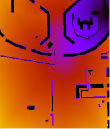
        Color - from blue to orange - indicates the length of
        the path traveled. We left the upper right corner.


Thus, we manage to limit ourselves to a minimum of memory for storing the wave perimeter. Even caching tiles is not necessary. We consider this option acceptable, and the goal of saving RAM has been achieved.

Fighting for disk memory

To store one tile of 256 × 256 points with a resolution of 1 bit per point, 8 kilobytes is required. Then a square kilometer costs 32 kilobytes, and a typical city with surroundings - 100 × 100 km already weighs 320 MB.

Too much. But this kind of information should be well compressed, since there are significant distortions in the ratio of 0 and 1. In addition, there are long monotonous sequences.

Initially, taking this into account, we used an adaptive arithmetic encoder. Rasterization of Novosibirsk took about four minutes. It turned out 4946 non-empty tiles, which took about 10 MB. At the same time, the same data in gifs takes up only 6 MB (which is humiliating :-). It looks like this:

        

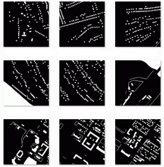
        Several arbitrary tiles in the form of pictures


10 or even 6 MB for Novosibirsk is more than our routing index takes.

In addition, if we go not from point to point, but to the road, then we need another raster - with roads that a pedestrian can reach. This is already too much. We found another solution - rasterization "on the fly."

On-the-fly rasterization

At first glance, this approach does not require additional information. In fact, we already have information: houses, fences, roads - with only a dozen layers.

But then, to rasterize each tile, you will have to make 10 spatial queries to spatial indices, followed by subtraction from the corresponding spatial layers.

With the limitations of the mobile phone on available memory, the data warehouse has almost no cache. And the subsystem is “alien” - we do not have a trusting relationship with it, therefore, memory is allocated through CRT, which is not very good from the point of view of fragmentation.

Simply put, this option is too expensive. So we made our data warehouse for rasterization.

For storing geometries, a B-tree is used with a key of 3 elements (or of two + value, if you like):

1. TileID - tile identifier. The extent of the map is divided into tiles, the numbering goes line by line from bottom to top from left to right.
2. Attr is an attribute of the object. We use only 1 least significant bit. 0 - we rasterize the object with ones, 1 - zeros.
   When traversing a tree, the zeros go forward, and we first draw all the blocking objects (houses, fences), and then apply resolving objects (wickets, transfers) on top.
3. Shp - geometry, all types of geometries are packed together.

Such an organization in one search and one traverse finds the data of this tile. In this case, mainly stack objects are used. Additional memory is taken from the pool, which is noticeably more humane in relation to CRT.

Geometries at the export stage are clipped along tile boundaries. When writing a tree, the data is compressed. As a result, storing vector information is three times more compact than rasterized when compared with an adaptive arithmetic encoder, and twice as economically as gif.

Route Examples

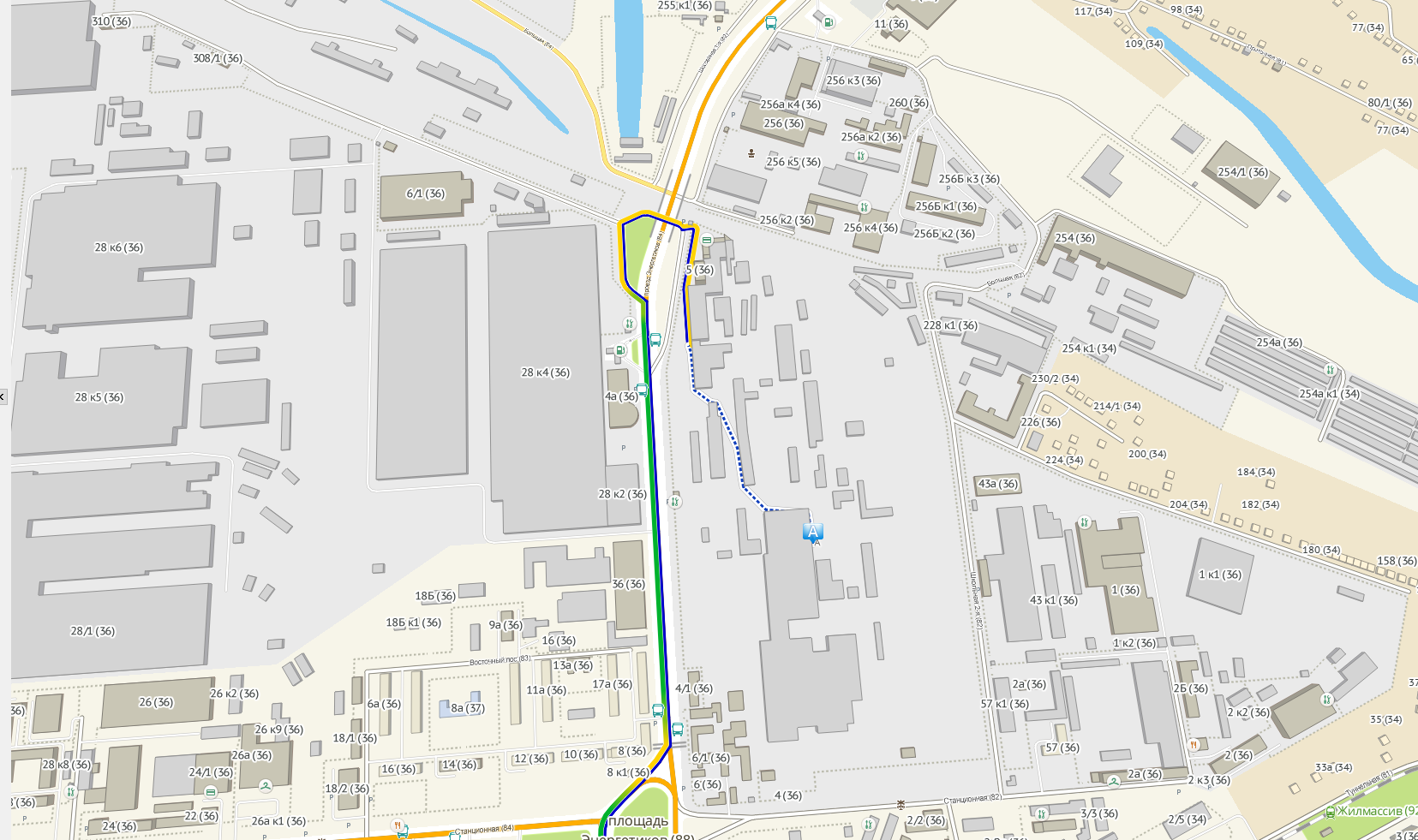
We go from point to point, pass through the railway station relocation.

        


Again from point to point. Sometimes the pedestrian path in the urban jungle is intricate.

        


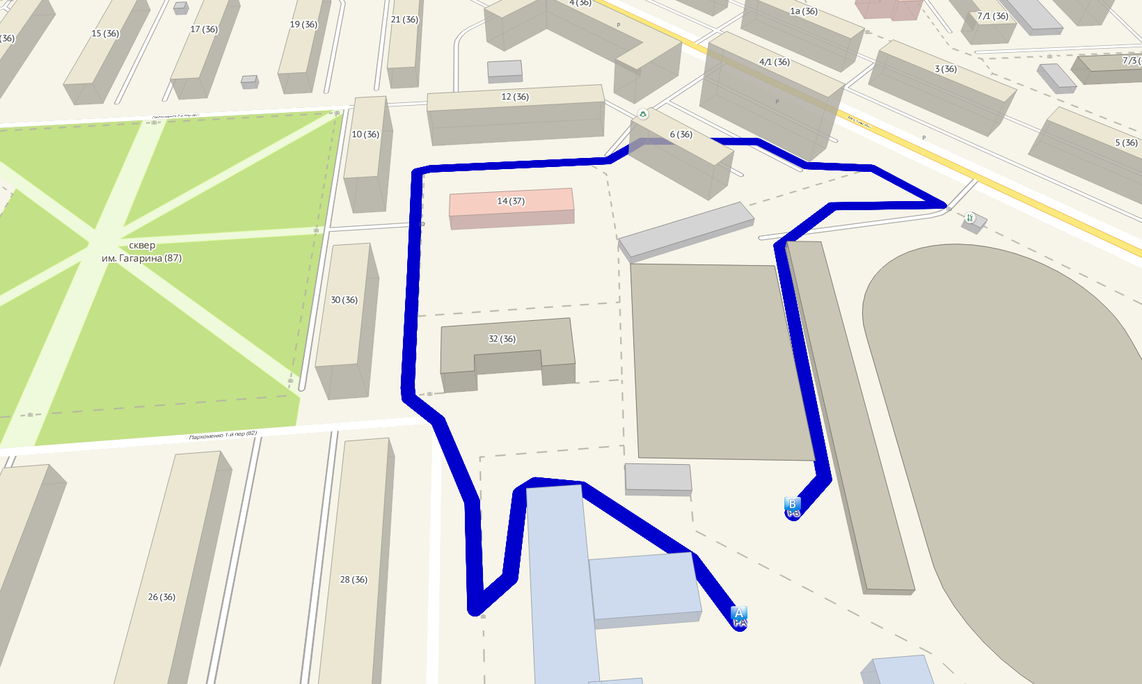
We go to the nearest road.

        


Again to the nearest rib.

        

What is the result

The amount of additional data for Novosibirsk is approximately 3 Mb. The capital of our vast Motherland is 8Mb. Searching for 1.5 km on the desktop takes 90 ms without warming up. These are about 20 unpacked and processed tiles. Additional RAM usually requires less than a megabyte.

But the approach has drawbacks. Despite the “straightening" of the geometries, sometimes the result is rather strange. For example, due to the discreteness of rasterization, buildings “stick together” from time to time.

The algorithm is quadratic to distance and nothing can be done with it. Fortunately, it is extremely rare to build at such distances when it becomes a problem. In fact, we limit the walking distance to two kilometers.

And yet, this is better than being attracted directly to the nearest roads and striding through cities and towns, despite obstacles. Hiking routes are already working in mobile apps on iOS, and Windows Phone and when searching for public transport on 2gis.ru .