Laplace Blur - Is it possible to blur Laplace instead of Gauss, how many times is it faster, and is it worth the loss of 1/32 accuracy

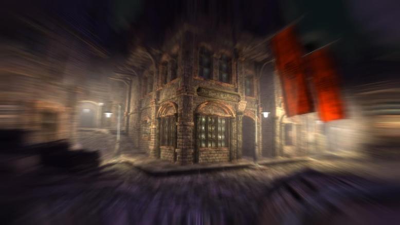
Blur in the common people - the effect of blurring, in digital image processing. It can be very effective both by itself and as a component of interface animations, or more complex derivative effects (bloom / focusBlur / motionBlur). With all this honest blur in the forehead rather slow. And often the implementations embedded in the target platform leave much to be desired. That speed is sad, then artifacts cut eyes. The situation gives rise to many compromise realizations, better or worse suitable for certain conditions. The original implementation with good quality of reliability and the highest speed, while the lowest dependence on the hardware is waiting for you under the cut. Enjoy your meal!

(Laplace Blur - The proposed original name of the algorithm)

Today, my internal demoscener kicked me and made me write an article that had to be written six months ago. As an amateur at leisure to develop original effect algorithms, I would like to propose to the public an “almost gaucian blura” algorithm, featuring the use of extremely fast processor instructions (shifts and masks), and therefore is available for implementation up to microcontrollers (extremely fast in a limited environment).

According to my tradition of writing articles on Habr, I will give examples in JS, as in the most popular language, and believe it or not, it is very convenient for the rapid prototyping of algorithms. In addition, the ability to implement this effectively on JS has come along with typed arrays. On my not very powerful laptop, the fullscreen image is processed at a speed of 30fps (the multithreading of the workers was not involved).


This description is present here rather to explain the course of my thoughts and conjectures that led me to the result. For those who will be interested in:

Original Gauss Function:



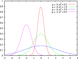
g (x) = a * e ** (- ((xb) ** 2) / c), where
a is the amplitude (if we have color eight bits per channel, then = 256)
e is the Euler constant ~ 2.7
b is the shift of the graph in x (we do not need = 0)
s is the parameter affecting the width of the graph associated with it as ~ w / 2.35

Our private function (minus from the exponent is removed with the substitution of multiplication by division ):



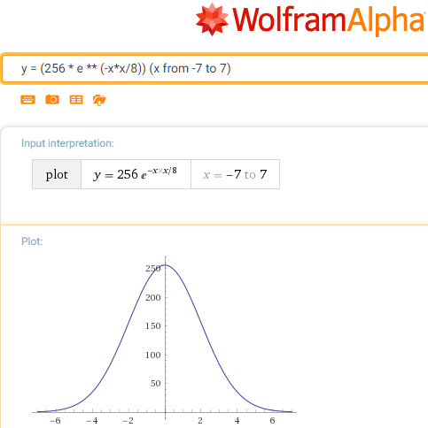
g (x) = 256 / e ** (x * x / c)

Let the dirty approximation action begin:
Note that the parameter c is very close to the half-width and set to 8 (this is due to how many steps you can move along one 8-bit channel).

We will also roughly replace e with 2, noting, however, that this affects the curvature of the “bell” more than its borders. Actually, it affects 2 / e times, but the surprise is that this error compensates for the parameter introduced in the definition of the parameter s, so that the boundary conditions are still in order, and the error appears only in a slightly incorrect “normal distribution”, for graphic algorithms, this will affect the dynamics of gradient color transitions, but it is almost impossible to notice with the eye.

So now our function is:
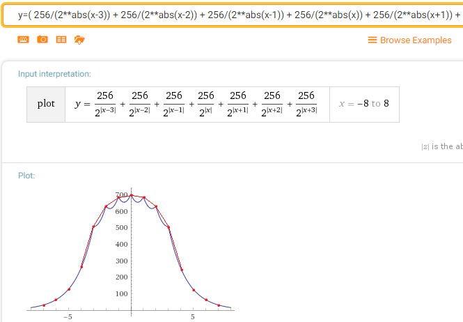
gg (x) = 256/2 ** (x * x / 8) or gg (x) = 2 ** (8 - x * x / 8)
Note that the exponent (x * x / 8) has the same range of values ​​[0-8] as the function of the smaller order abs (x), because the latter is a candidate for replacement. Quickly check the guess by looking at how the graph changes with it gg (x) = 256 / (2 ** abs (x)):

GaussBlur vs LaplasBlur:



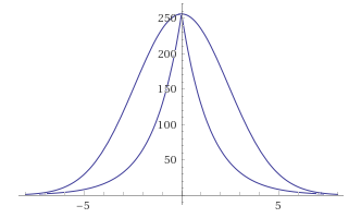
It seems the deviations are too large, besides, the function, having lost its smoothness, now has a peak. But wait.

First, let us not forget that the smoothness of the gradients obtained by blurring does not depend on the probability density function (which is the Gauss function), but on its integral — the distribution function. At that moment I did not know this fact, but in fact, after conducting a “destructive” approximation with respect to the probability density function (Gauss), the distribution function remained quite similar.

It was:



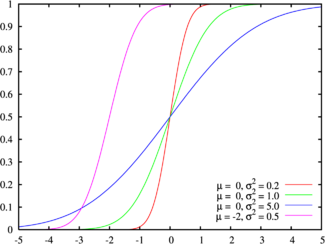
It became:



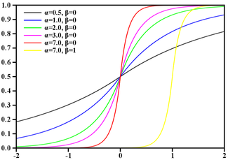
Proof, taken from the finished algorithm, coincides:



(looking ahead, I will say that the blur error of my algorithm relative to Gausian x5 was only 3%).

So, we have moved much closer to the Laplace distribution function. Who would have thought, but they can wash images at 97% no worse.

Proof, the differences of the Gaucian Blura x5 and “Laplace Blura” x7:



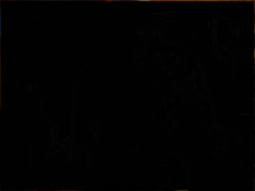
(this is not a black image! You can study in the editor) The

admission of this transformation made it possible to proceed to the idea of ​​obtaining the value by iterative filtering, which I planned to reduce to the beginning.

Before the narration of a specific algorithm, it will be fair if I run ahead and immediately describe its only drawback (although the implementation can be fixed, with a loss of speed). But this algorithm is implemented using shear arithmetic, and degrees 2k are its limitation. So the original is made to blur x7 (which in the tests is the closest to the Gausian x5). This implementation restriction is related to the fact that with eight-bit color, shifting the value in the filter drive by one bit per step, any effect from a point ends in a maximum of 8 steps. I also implemented a slightly slower version in terms of proportions and additional additions, which realizes a fast division by 1.5 (having obtained as a result a radius of x15). But with the further application of this approach, the error increases, and the speed drops, which does not allow using it so. On the other hand, it is worth noting that x15 is already enough to not notice much of the difference, the result is obtained from the original or from the downsampled image. So the method is quite suitable if you need extreme speed in a limited environment.

So, the core of the algorithm is simple, four passes of the same type are performed:

1. Half of the value of drive t (initially equal to zero) is added to half of the value of the next pixel, the result is assigned to it. We continue this way until the end of the image line. For all lines.

Upon completion of the first pass, the image is blurred in one direction.

2. Use the second pass to do the same for all lines.
We get the image completely blurred horizontally.

3-4. Now do the same thing vertically.
Done!

Initially, I used a two-pass algorithm with the implementation of reverse blurring through the stack, but it is difficult to understand, not graceful, and besides, on the current architectures it turned out to be slower. Perhaps the one-pass algorithm will be faster on microcontrollers, plus it will also be possible to output the result progressively.

The current four-pass method of implementation, I peeped on Habré from the previous guru on blur algorithms. habr.com/post/151157 Taking this opportunity, I express my solidarity and deep gratitude to him.

But the hacks didn't end there. Now, about how to calculate all three color channels for one processor instruction! The fact is that the bit shift used as a division by two allows the position bits of the result to be very well controlled. The only problem is that the lower bits of the channels slide into the neighboring older ones, but you can simply reset them, rather than correct the problem, with some loss of accuracy. And according to the described filter formula, the addition of half the value of the drive with half the value of the next cell (assuming zeroing of the discharged discharges) never leads to overflow, so you should not worry about it. And the filter formula for the simultaneous calculation of all digits becomes:

buf32 [i] = t = (((t >> 1) & 0x7F7F7F) + ((buf32 [i] >> 1) &

However, another addition is required: it was empirically found that the loss of accuracy in this formula is too significant, the brightness of the picture visually jumps noticeably. It became clear that the lost bits should be rounded to the whole, and not discarded. A simple way to do this in integer arithmetic is to add half the divider before division. The divider is a two for us, so you need to add one, in all digits, - the constant 0x010101. But with any addition you need to be careful not to get overflow. So we cannot use this correction to calculate the half value of the next cell. (If there is a white color, we will get an overflow, therefore we will not correct it). But it turned out that the main mistake was made by the multiple division of the drive, which we can correct. Because, in fact, even with such a correction, the value in the accumulator will not rise above 254. But when combined with 0x010101, the overflow will not be guaranteed. And the filter formula with correction takes the form:

buf32 [i] = t = ((((0x010101 + t) >> 1) & 0x7F7F7F) + ((buf32 [i] >> 1) & 0x7F7F7F);

In fact, the formula performs a good enough correction, so with repeated Repeated application of the algorithm to the image, artifacts begin to be seen only in the second ten or so passes. (It’s not a fact that repeating the Ghusian Blur will not give such artifacts.)

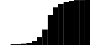
Additionally, there is a remarkable property, with many passes. (It is not the merit of my algorithm, but the “normal "Normal distribution.) Already on the second pass Laplace Blur function density of faith



To the best of my knowledge (if I figured it all out correctly) it will look something like this: That, you see, is already very close to the Gaussian.

Experimentally, I have found that it is permissible to use modifications with a large radius as a pair, since The property described above compensates for errors if the last pass is more accurate (the most accurate one is the x7 blur algorithm described here).

demo
rep
kodpen

Appeal for cool mathematicians:
What would be interesting to know how well to use such a filter is separable, not sure if there is a symmetrical distribution pattern. Although the eye of heterogeneity and is not visible.

upd: Here I will raise useful links, courtesy presented by commentators, and found in other habrovchan.
1. How do intel masters work, relying on the power of SSE -software.intel.com/en-us/articles/iir-gaussian-blur-filter-implementation-using-intel-advanced-vector-extensions (thanks to vladimirovich )
2. Theoretical base on the topic “Fast image convolutions” + some of its custom applications with respect to fair Ghusian Blurals - blog.ivank.net/fastest-gaussian-blur.html (thanks to Grox )

Suggestions, comments, constructive criticism are welcome!