How to find out the year of release of a song by a set of audio characteristics?
- From the sandbox
- Tutorial
The Scalable Machine Learning course on Apache Spark, which talks about using the MLlib library for machine learning, has recently completed . The course consisted of video lectures and practical exercises. Laboratory work had to be done on PySpark, and since I often have to deal with scala for work, I decided to re-fix the main labs in this language, and at the same time it’s better to learn the material. Of course there are no big differences, basically, it is that PySpark actively uses NumPy , and in the version with scala Breeze is used .
The first two hands-on classes covered learning the basic operations of linear algebra in NumPy and getting to know apache spark, respectively. Actually machine learning began with the third laboratory work, and it is disassembled below.
This laboratory work is aimed at studying the linear regression method (one of the teaching methods with a teacher). We will use part of the data from the Million Song Dataset . Our goal is to find the best model that predicts the year of a song by a set of audio characteristics using the linear regression method.
This lab includes the following steps:
1. Reading, parsing and processing data
2. Creating and evaluating the base model
3. Implementing the basic linear regression algorithm, training and evaluating the model
4. Finding the model using MLlib, setting up hyper parameters
5. Adding dependencies between characteristics
The raw data is currently stored in a text file and consists of lines of the following form:
Each line starts with a label (year of release of the song), and then the audio characteristics of the recording, separated by a comma, follow.
The first thing we will start with: present the data as an RDD:
Let's see how many records we have:
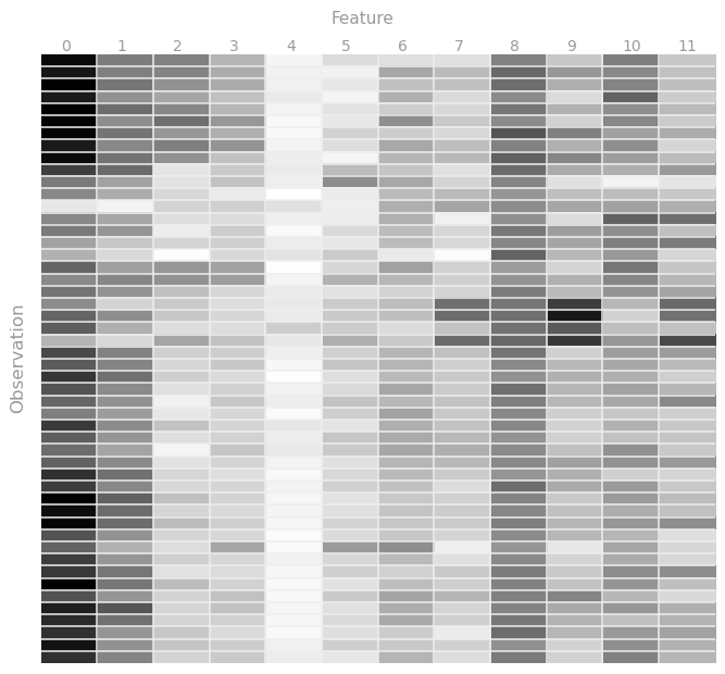
In order to better understand the data provided to us, let's visualize them by constructing a heat map for at least part of the observations. Because Since the characteristics are in the range from 0 to 1, then let the closer the value to unity the darker the shade of gray will be, and vice versa.
In MLlib, the training set (more precisely, its elements) must be stored in a special LabeledPoint object , which consists of a label and a set of features belonging to this label. In our case, the label will be the year, and the characteristics are the audio data of the recording.
We will write a function that will receive one row from our data set at the input and return the finished labeledPoint.
We translate our data into a working version:
Now let's examine the labels and find the range of years that our data fits into; To do this, you need to find the maximum and minimum year.
As we can see, the labels are located between 1922 and 2011. In learning tasks, it is often natural to shift values so that they start from scratch. Let's create a new RDD that will contain objects with tags offset by 1922.0.
We have almost finished preparing the data, and all that remains for us is to split the data into 3 subsets:
For these purposes, spark has a randomSplit method :
Let's try to come up with a simple model with which we could compare the accuracy of the models obtained in the future. In the simplest case, the model can give as a prediction the average value of the year, regardless of the input data. Let's calculate this value:
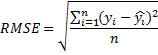
To evaluate how well our model works, let's use the square root of the mean square error ( RMSE ) as an estimate
 .
.
In our case, y i is the year label, and y i with a cap is the year predicted by the model. First, we implement a function that computes the square of the difference between label and prediction and a function that will calculate RMSE:
Now we can calculate the RMSE of our data based on the predictions of the underlying model. To do this, prepare new RDD containing tuples with observed and forecast years.
Note that each RMSE received can be interpreted as the average forecast error for a given set (in terms of the number of years)
Now that we have the basic model and its assessment, we can check whether the linear regression method can offer us a better result than the previous one.
Recall the gradient descent step formula for linear regression:
w i + 1 = w i - α i * ∑ (w i T * x j - y j ) * x j .
Where i is the iteration number and j is the observation identifier.
First, we implement a function that calculates the term for this update (w T * x - y) * x:
We go further: we need to implement a function that will take the calculated model weights and observed values, and give it a tuple (observed value, predicted value).
It is time to implement the Gradient Descent method:
Well, everything is ready! Now it remains to train our linear regression model on the entire training sample and evaluate its accuracy on the test sample:
At each iteration, we counted the RMSE for the training sample and now we can track how the algorithm behaved: for this we construct two graphs. The first is the logarithm of the error from the iteration number for all 50 iterations, and the second is the actual error value for the last 44 iterations.

We clearly achieved improvements: now our predictions are mistaken, on average, not by 21 years, but by only 18. It should be noted that if the number of iterations is increased to 500, the error will be 16,403.
Well, now it looks much better. However, let's see if we can improve the situation using the free term (constant, intercept) and regularization. To do this, we will use the ready-made LinearRegressionWithSGD class, which essentially implements the same algorithm that we implemented, but more efficiently, with various additional functionality, such as, for example, stochastic gradient descent, the possibility of adding a free term, and also L1 and L2 regularization.
To begin with, we implement a function that will help you configure the model:
We used RidgeRegressionWithSGD, because it is a wrapper with an already defined type of regularization L2, just as we could use LinearRegressionWithSGD, but then we would have to add another line
Run the algorithm:
The result is comparable to our implementation (and if you recall that with an equal number of iterations we got 16.4, then the result is not so hot), but, probably, we can improve the result by trying different regularization values. Let's see what happens if we take the regularization parameter 1e-10, 1e-5 and 1.
It remains to verify how the model behaves if we change the value of the step (alpha) and the number of iterations. We take the regularization parameter that gave the best value, let the step be 1e-5, 10, and the number of iterations 500 and 5.
So, we can conclude that with a small step, the algorithm very slowly approaches a minimum, and with a large step it generally diverges, moreover, very quickly.
So far, we have used only those characteristics that were provided to us. For example, if we had only 2 characteristics x 1 and x 2 , then the model would be:
w 0 + w 1 x 1 + w 2 x 2 .
However, nothing prevents us from creating additional characteristics: returning to our example, we could come up with a more complicated model:
w 0 + w 1 x 1 + w 2 x 2 + w 3 x 1 x 2 + w 4 x 2x 1 + w 5 x 1 2 + w 6 x 2 2
Let's do this; for this we need to implement a function that multiplies the values of the characteristics in pairs and returns a new set, combined with the original one.
Now let's create a new model, for this we need to apply the function described above to our data sets:
Well, then we must repeat the search for hyperparameters for the new model, because the settings found earlier may not give the best result. But we will not repeat this here, but immediately substitute the optimal ones.
And finally, we will evaluate our new model on test data. Please note that we did not use test data to select the best model. Therefore, our assessment gives an unbiased assessment of how the resulting model will work on new data. Now we can see how much the new model is better than the base.
Well, that's all, the final assessment certainly does not look particularly good, but definitely better than the one with which we started.
The first two hands-on classes covered learning the basic operations of linear algebra in NumPy and getting to know apache spark, respectively. Actually machine learning began with the third laboratory work, and it is disassembled below.
This laboratory work is aimed at studying the linear regression method (one of the teaching methods with a teacher). We will use part of the data from the Million Song Dataset . Our goal is to find the best model that predicts the year of a song by a set of audio characteristics using the linear regression method.
This lab includes the following steps:
1. Reading, parsing and processing data
2. Creating and evaluating the base model
3. Implementing the basic linear regression algorithm, training and evaluating the model
4. Finding the model using MLlib, setting up hyper parameters
5. Adding dependencies between characteristics
1. Reading, parsing and data processing
The raw data is currently stored in a text file and consists of lines of the following form:
2001.0,0.884123733793,0.610454259079,0.600498416968,0.474669212493,0.247232680947,0.357306088914,0.344136412234,0.339641227335,0.600858840135,0.425704689024,0.60491501652,0.419193351817
Each line starts with a label (year of release of the song), and then the audio characteristics of the recording, separated by a comma, follow.
The first thing we will start with: present the data as an RDD:
  val sc = new SparkContext("local[*]", "week3")
  val rawData: RDD[String] = sc.textFile("millionsong.txt")
Let's see how many records we have:
  val numPoints = rawData.count()
  println(numPoints)
  > 6724
In order to better understand the data provided to us, let's visualize them by constructing a heat map for at least part of the observations. Because Since the characteristics are in the range from 0 to 1, then let the closer the value to unity the darker the shade of gray will be, and vice versa.
In MLlib, the training set (more precisely, its elements) must be stored in a special LabeledPoint object , which consists of a label and a set of features belonging to this label. In our case, the label will be the year, and the characteristics are the audio data of the recording.
We will write a function that will receive one row from our data set at the input and return the finished labeledPoint.
  import org.apache.spark.mllib.regression.LabeledPoint
  import org.apache.spark.mllib.linalg.Vectors
  def parsePoint(line: String) = {
    val sp = line.split(',')
    LabeledPoint(sp.head.toDouble, Vectors.dense(sp.tail.map(_.toDouble)))
  }
We translate our data into a working version:
val parsedDataInit: RDD[LabeledPoint] = rawData.map(parsePoint)
Now let's examine the labels and find the range of years that our data fits into; To do this, you need to find the maximum and minimum year.
  val onlyLabels = parsedDataInit.map(_.label)
  val minYear = onlyLabels.min()
  val maxYear = onlyLabels.max()
  println(s"max: $maxYear, min: $minYear")
  > max: 2011.0, min: 1922.0
As we can see, the labels are located between 1922 and 2011. In learning tasks, it is often natural to shift values so that they start from scratch. Let's create a new RDD that will contain objects with tags offset by 1922.0.
val parsedData = parsedDataInit.map(x => LabeledPoint(x.label - minYear, x.features))
We have almost finished preparing the data, and all that remains for us is to split the data into 3 subsets:
- training sample - it is on it that we will train our model
- test sample - on this data we will check how successfully trained model predicts the result
- test sample - this set will simulate new data and will help us to truly evaluate the best model
For these purposes, spark has a randomSplit method :
  val weights = Array(0.8, 0.1, 0.1)
  val seed = 42
  val splitData: Array[RDD[LabeledPoint]] = parsedData.randomSplit(weights, seed).map(_.cache())
  val parsedTrainData = splitData(0)
  val parsedValData = splitData(1)
  val parsedTestData = splitData(2)
  val nTrain = parsedTrainData.count()
  val nVal = parsedValData.count()
  val nTest = parsedTestData.count()
  println(nTrain, nVal, nTest, nTrain + nVal + nTest)
  println(parsedData.count())
  >(5402,622,700,6724)
  > 6724
2. Creation and evaluation of the base model
Let's try to come up with a simple model with which we could compare the accuracy of the models obtained in the future. In the simplest case, the model can give as a prediction the average value of the year, regardless of the input data. Let's calculate this value:
  val averageTrainYear = parsedTrainData.map(_.label).mean()
  println(averageTrainYear)
  > 53.68659755646054
To evaluate how well our model works, let's use the square root of the mean square error ( RMSE ) as an estimate
. In our case, y i is the year label, and y i with a cap is the year predicted by the model. First, we implement a function that computes the square of the difference between label and prediction and a function that will calculate RMSE:
  def squaredError(label: Double, prediction: Double) = math.pow(label - prediction, 2)
  def calcRMSE(labelsAndPreds: RDD[(Double, Double)]) =
    math.sqrt(labelsAndPreds.map(x => squaredError(x._1, x._2)).sum() / labelsAndPreds.count())
Now we can calculate the RMSE of our data based on the predictions of the underlying model. To do this, prepare new RDD containing tuples with observed and forecast years.
  val labelsAndPredsTrain = parsedTrainData.map(x => x.label -> averageTrainYear)
  val rmseTrainBase = calcRMSE(labelsAndPredsTrain)
  val labelsAndPredsVal = parsedValData.map(x => x.label -> averageTrainYear)
  val rmseValBase = calcRMSE(labelsAndPredsVal)
  val labelsAndPredsTest = parsedTestData.map(x => x.label -> averageTrainYear)
  val rmseTestBase = calcRMSE(labelsAndPredsTest)
  > Base model:
	Baseline Train RMSE = 21,496
	Baseline Validation RMSE = 21,100
	Baseline Test RMSE = 21,100
Note that each RMSE received can be interpreted as the average forecast error for a given set (in terms of the number of years)
3. Implementation of the basic linear regression algorithm, training and model estimation
Now that we have the basic model and its assessment, we can check whether the linear regression method can offer us a better result than the previous one.
Recall the gradient descent step formula for linear regression:
w i + 1 = w i - α i * ∑ (w i T * x j - y j ) * x j .
Where i is the iteration number and j is the observation identifier.
First, we implement a function that calculates the term for this update (w T * x - y) * x:
  import breeze.linalg.{ DenseVector => BreezeDenseVector }
  def gradientSummand(weights: BreezeDenseVector[Double], lp: LabeledPoint): BreezeDenseVector[Double] = {
    val x = BreezeDenseVector(lp.features.toArray)
    val y = lp.label
    val wx: Double = weights.t * x
    (wx - y) * x
  }
We go further: we need to implement a function that will take the calculated model weights and observed values, and give it a tuple (observed value, predicted value).
  def getLabeledPrediction(weights: BreezeDenseVector[Double], observation: LabeledPoint): (Double, Double) = {
    val x = BreezeDenseVector(observation.features.toArray)
    val y = observation.label
    val prediction: Double = weights.t * x
    (y, prediction)
  }
It is time to implement the Gradient Descent method:
  def linregGradientDescent(trainData: RDD[LabeledPoint], numIters: Int) = {
    // Размер обучающей выборки
    val n = trainData.count()
    // Кол-во характеристик
    val d = trainData.first().features.size
    // Создаём начальный вектор весов (состоит из d нулей)
    val w = BreezeDenseVector.zeros[Double](d)
    val alpha = 1.0
    val errorTrain = BreezeDenseVector.zeros[Double](numIters)
    for (i <- 0 until numIters) {
      val labelsAndPredsTrain = trainData.map(x => getLabeledPrediction(w, x))
      errorTrain(i) = calcRMSE(labelsAndPredsTrain)
      val gradient: BreezeDenseVector[Double] = trainData.map(x => gradientSummand(w, x)).reduce((dv1, dv2) => dv1 + dv2)
      val alpha_i = alpha / ( n * math.sqrt(i+1) )
      w -= alpha_i * gradient
    }
    (w, errorTrain)
  }
Well, everything is ready! Now it remains to train our linear regression model on the entire training sample and evaluate its accuracy on the test sample:
  val numIters = 50
  val (weightsCustom, errorTrainCustom) = linregGradientDescent(parsedTrainData, numIters = numIters)
  val labelsAndPreds = parsedValData.map(lp => getLabeledPrediction(weightsCustom, lp))
  val rmseValLRCustom = calcRMSE(labelsAndPreds)
  > Custom Linear regression algorithm
	Weights = DenseVector(22.429559050840954, 20.57848949803509, -0.38069311013701224, 8.286892767462648, 5.725188813272974, -4.547779089973534, 15.494323154076804, 3.7888305696294986, 10.205862111138764, 5.877745123091225, 11.13061973187094, 3.6849419014146703)
	Baseline = 21,100
	CustomLR = 18,341
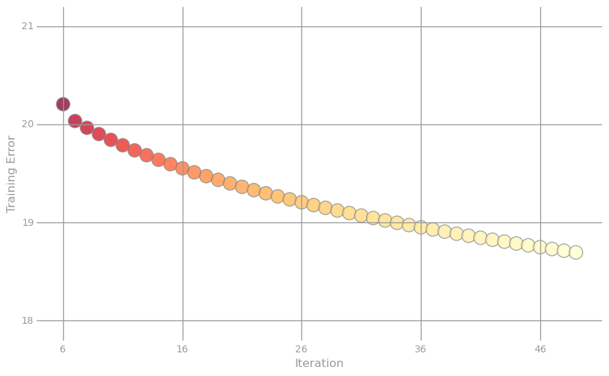
At each iteration, we counted the RMSE for the training sample and now we can track how the algorithm behaved: for this we construct two graphs. The first is the logarithm of the error from the iteration number for all 50 iterations, and the second is the actual error value for the last 44 iterations.
We clearly achieved improvements: now our predictions are mistaken, on average, not by 21 years, but by only 18. It should be noted that if the number of iterations is increased to 500, the error will be 16,403.
4. Finding a model using MLlib, setting hyperparameters
Well, now it looks much better. However, let's see if we can improve the situation using the free term (constant, intercept) and regularization. To do this, we will use the ready-made LinearRegressionWithSGD class, which essentially implements the same algorithm that we implemented, but more efficiently, with various additional functionality, such as, for example, stochastic gradient descent, the possibility of adding a free term, and also L1 and L2 regularization.
To begin with, we implement a function that will help you configure the model:
  import org.apache.spark.mllib.regression.RidgeRegressionWithSGD
  def tuneModel(numIterations: Int = 500, stepSize: Double = 1.0, regParam: Double = 1e-1) = {
    val model = new RidgeRegressionWithSGD()
    model.optimizer
      .setStepSize(stepSize)
      .setNumIterations(numIterations)
      .setRegParam(regParam)
    model.setIntercept(true)
  }
We used RidgeRegressionWithSGD, because it is a wrapper with an already defined type of regularization L2, just as we could use LinearRegressionWithSGD, but then we would have to add another line
model.optimizer.setUpdater(new SquaredL2Updater)Run the algorithm:
  val ridgeModel = tuneModel(numIterations = 500, stepSize = 1.0, regParam = 1e-1).run(parsedTrainData)
  val weightsRidge = ridgeModel.weights
  val interceptRidge = ridgeModel.intercept
  val rmseValRidge = calcError(ridgeModel, parsedValData)
  > RidgeRegressionWithSGD
	weights = [16.49707401343799,15.090143596016913,-0.33882414671890876,6.21399054657087,3.9399959912276765,-3.326873353072514,11.219894673155363,2.605614334247694,7.368594539065305,4.352602095699236,7.936294197372791,2.597979499976716]
	intercept = 13.40151357030002
  > RidgeRegressionWithSGD validation RMSE
	Baseline = 21,100
	CustomLR = 18,341
	RidgeLR = 18,924
The result is comparable to our implementation (and if you recall that with an equal number of iterations we got 16.4, then the result is not so hot), but, probably, we can improve the result by trying different regularization values. Let's see what happens if we take the regularization parameter 1e-10, 1e-5 and 1.
  var bestRMSE = rmseValRidge
  var bestRegParam = 1.0
  var bestModel = ridgeModel
  for (regParam <- Array(1e-10, 1e-5, 1)) {
    val model = tuneModel(regParam = regParam).run(parsedTrainData)
    val rmseVal = calcError(model, parsedValData)
    println(f"regParam = $regParam%.0e, RMSE = $rmseVal%.3f")
    if (rmseVal < bestRMSE) {
      bestRMSE = rmseVal
      bestRegParam = regParam
      bestModel = model
    }
  }
  > regParam = 1e-10, RMSE = 16,292
     regParam = 1e-05, RMSE = 16,292
     regParam = 1e+00, RMSE = 23,179
  > Best model
	weights = [29.417184432817606,31.186800575308965,-17.37215928935944,8.288971260120093,5.111705048981693,-22.61199371516979,25.231243109503467,-4.989933439427709,6.709806469376133,-0.08589332350175394,9.958713420381914,-6.252319073419468]
	intercept = 16.170147238736043
	regParam = 1.0E-10
  > Grid validation RMSE
	Baseline = 21,100
	LR0 = 18,341
	LR1 = 18,924
	LRGrid = 16,292
It remains to verify how the model behaves if we change the value of the step (alpha) and the number of iterations. We take the regularization parameter that gave the best value, let the step be 1e-5, 10, and the number of iterations 500 and 5.
  for (alpha <- Array(1e-5, 10)) {
    for (numIter <- Array(5, 500)) {
      val model = tuneModel(numIterations = numIter, stepSize = alpha, regParam = bestRegParam).run(parsedTrainData)
      val rmseVal = calcError(model, parsedValData)
      println(f"alpha = $alpha%.0e, numIters = $numIter, RMSE = $rmseVal%.3f")
    }
  }
  > alpha = 1e-05, numIters = 5,   RMSE = 56,912
    alpha = 1e-05, numIters = 500, RMSE = 56,835
    alpha = 1e+01, numIters = 5,   RMSE = 351471078,741
    alpha = 1e+01, numIters = 500, RMSE = 3696615731186115000000000000000000000000000000000000000000000000000000000000000000000000000000000000000000000000000000000,000
So, we can conclude that with a small step, the algorithm very slowly approaches a minimum, and with a large step it generally diverges, moreover, very quickly.
5. Adding dependencies between characteristics
So far, we have used only those characteristics that were provided to us. For example, if we had only 2 characteristics x 1 and x 2 , then the model would be:
w 0 + w 1 x 1 + w 2 x 2 .
However, nothing prevents us from creating additional characteristics: returning to our example, we could come up with a more complicated model:
w 0 + w 1 x 1 + w 2 x 2 + w 3 x 1 x 2 + w 4 x 2x 1 + w 5 x 1 2 + w 6 x 2 2
Let's do this; for this we need to implement a function that multiplies the values of the characteristics in pairs and returns a new set, combined with the original one.
  def twoWayInteractions(lp: LabeledPoint) = {
    val features: List[Double] = lp.features.toArray.toList
    val two = (for (x <- features; y <- features) yield (x,y)).map(x => x._1 * x._2)
    val inter = two ::: features
    LabeledPoint(lp.label, Vectors.dense(inter.toArray))
  }
Now let's create a new model, for this we need to apply the function described above to our data sets:
  val trainDataInteract = parsedTrainData.map(twoWayInteractions)
  val valDataInteract = parsedValData.map(twoWayInteractions)
  val testDataInteract = parsedTestData.map(twoWayInteractions)
Well, then we must repeat the search for hyperparameters for the new model, because the settings found earlier may not give the best result. But we will not repeat this here, but immediately substitute the optimal ones.
  val modelInteract = tuneModel(regParam = bestRegParam).run(trainDataInteract)
  val rmseValLRInteract = calcError(modelInteract, valDataInteract)
  > Interact validation RMSE
	Baseline = 21,100
    LR0 = 18,341
	LR1 = 18,924
	LRGrid = 16,292
	LRInteract = 15,225
And finally, we will evaluate our new model on test data. Please note that we did not use test data to select the best model. Therefore, our assessment gives an unbiased assessment of how the resulting model will work on new data. Now we can see how much the new model is better than the base.
  > Test validation RMSE
	Baseline = 21,100
	LRInteract = 15,905
Well, that's all, the final assessment certainly does not look particularly good, but definitely better than the one with which we started.