Content

1. What is a tensor and why is it needed?
2. Vector and tensor operations. Tensor Ranks
3. Curvilinear coordinates
4. The dynamics of a point in tensor exposition
5. Actions on tensors and some other theoretical questions
6. Kinematics of a free solid. The nature of angular velocity
7. The final rotation of a solid. Properties of the rotation tensor and method of its calculation
8. On convolutions of the Levi-Civita tensor
9. The derivation of the angular velocity tensor through the parameters of the final rotation. Apply the head and Maxima
10. We get the angular velocity vector. Working on shortcomings
11. Acceleration of a body point in free movement. Angular acceleration of a solid
12. Rodrigue Hamilton Parameters in Solid State Kinematics
13. SKA Maxima in problems of transformation of tensor expressions. Angular velocity and acceleration in the parameters of Rodrigue Hamilton
14. Non-standard introduction to the dynamics of a rigid body
15. Proprietary Solid Motion
16. Properties of the inertia tensor of a solid
17. Sketch of a nut Janibekova
18. Mathematical modeling of the Janibekov effect

Introduction

In this article we will solve two issues - we will obtain expressions for the angular velocity and angular acceleration through the Rodrigue-Hamilton parameters, which we discussed in more detail than planned in the previous article . And at the same time, we will demonstrate how to use the open Maxima SKA for this purpose, which, as it turned out, copes well with tensors, and if there are certain skills, it can become a serious help in solving scientific problems. For me, Maxima is a new product, before that I worked with Maple and quite a bit with Mathematica. Therefore, perhaps some of the tricks I use may seem unprofessional.


SKA is ready to help us and is waiting for a reasonable team ...


Last time, we focused on showing how the quaternion algebra can be used to represent a rotation transformation. Knowing the direction of the rotation axis specified by the unit vector and the angle by which the coordinate system must be rotated, we can construct a unit quaternion with respect to the components

and then, the direct transformation of the rotation of the vector is reduced to the multiplication of quaternions

and the inverse transformation

We have shown that the transformations (2) and (3) carried out on the vector directly give the Rodrigue formula describing the final rotation. Now our goal is to connect the rotation quaternion parameters with the rotation tensor and pseudo-vectors of angular velocity and angular acceleration.

1. The rotation tensor in the parameters of Rodrigue Hamilton

We are already familiar with the expression for the rotation tensor



We introduce the quaternion, presenting its vector part as contravariant components



In this case, the substitution of (5) into (4) can be done manually; this process does not involve anything extraordinary. But we will do everything in Maxima, at the same time having prepared some initial data for further work. We configure Maxima to work with tensors in three-dimensional space

/* Очищаем память */
kill(all);
/* Загружаем пакеты для работы с тензорами и генерации LaTeX вывода */
load(itensor);
load(tentex);
/* Даем имя метрическому тензору и задаем размерность пространства */
imetric(g);
idim(3);

We introduce the expression (4) of the rotation tensor

B:ishow(2*sin(phi/2)^2*u([],[m])*u([k],[]) + 
(cos(phi/2)^2 - sin(phi/2)^2)*kdelta([k],[m]) + 
2*sin(phi/2)*cos(phi/2)*g([],[m,i])*'levi_civita([i,j,k],[])*u([],[j]))$

Pay attention to the nuance - we moved to the half corners. Otherwise, when trying to simplify trigonometry, Maxima will not simplify anything, even setting a flag halfanglesthat includes accounting for half-argument formulas does not help . This is the first crutch that I had to apply. Perhaps out of ignorance.

We set the relationship between the parameters of the final rotation and the components of the quaternion

Lambda0:p0 = cos(phi/2);
Lambda:ishow(p([],[j]) = sin(phi/2)*u([],[j]))$

Here, for brevity (laziness to enter each time lambda), the components of the quaternion are indicated by the letter p

Express the unit axis of the rotation axis through the vector part of the quaternion

Solv1:ishow(solve(Lambda, u([],[j])))$

getting the solution at the output of the equation in the form of an array of expressions



In the resulting expression, it is necessary to omit the index, since the rotation tensor contains the covariant components of the rotation unit vector. To do this, we collapse the expression obtained before this with the metric tensor

u_k:ishow(contract(Solv1[1]*g([k,j],[])))$

In addition, we replace the index j by m in the covariant components

um:ishow(subst(m, j, Solv1[1]))$

As a result, we obtain two expressions ready for substitution into the rotation tensor.



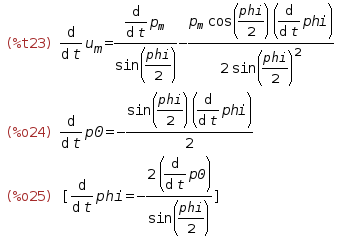
Now we can substitute the components of the orth of the rotation axis into the expression for the rotation tensor. The setting function subst()in this case takes two arguments - an expression that must be substituted into the expression that comes with the second argument. In this case, the left part of the first argument is searched in the converted expression and replaced with its right part

B_1:ishow(subst(u_k, B))$
B_1:ishow(subst(um, B_1))$
B_1:ishow(subst(Solv1[1], B_1))$

At the output we have



Excellent, now the components of the vector part of the quaternion appear in the rotation tensor. Now simplify trigonometry

B_2:ishow(trigsimp(B_1))$

The function trigsim()simplifies trigonometric expressions. Moreover, as written in the documentation, it takes into account by default the main trigonometric identity and the evenness / oddness of trigonometric functions. However, whether loading the tensor algebra package has such an effect, this function stumbles on the simplification of fractions containing the functions of single and half arguments, even when the flag mentioned above is cocked. Nevertheless, we did some preparatory work and at the end we get a simplified formula. It



remains to replace the squares of the cosine and sine of the half-angle of rotation with the scalar parameter of the quaternion, for which we perform the substitution and simplification in the form of opening brackets

B_3:ishow(subst(p0,rhs(Lambda0), B_2))$
B_3:ishow(expand(subst(1-p0^2,sin(phi/2)^2, B_3)))$

And to admire the result, we will output it in LaTeX

tentex(B_3);

To the output code, I added only the left part



It can be seen that Maxima generates LaTeX notation, which is very close to the natural mathematical notation, but the same cannot be said for Maple, which prepares a monstrous code containing all the conventions adopted by it in the derivation of readable formulas. The terms containing the Kronecker delta are grouped and the common factor is bracketed by ourselves. Well, back to the place of "lambda"



We have obtained the expression of the rotation tensor in terms of the Rodrig-Hamilton parameters. From this tensor, one can go to any other parameters describing the orientation of a rigid body in space.

The warm-up can be considered over. More serious work awaits us

2. Pseudovector of angular velocity in the parameters of Rodrigue Hamilton

We introduce into Maxima the expression we already know for the pseudovector of angular velocity. In natural form, it looks like this



And in Maxima it will go with the replacement of single-angle functions by equivalent half-functions

Omega:ishow(2*sin(phi/2)^2*'levi_civita([],[i,m,r])*u([i],[])*diff(u([m],[]),t) + 
diff(u([],[r]),t)*2*sin(phi/2)*cos(phi/2) + u([],[r])*diff(phi, t))$

Let me remind you that the Levi-Civita tensor, especially if you plan to simplify the expression using its properties, it is better to introduce with the suppression of the calculation. Otherwise, Maxima will turn it into a generalized Kronecker delta, and this is not included in our plans. To suppress the calculation, put an apostrophe in front of the name of the function that defines this tensor.

We omit the indices and rename the indices of the rotation unit vector, in accordance with the designation of the indices in the angular velocity tensor

u_i:ishow(contract(Solv1[1]*g([i,j],[])))$
u_m:ishow(subst(m, i, u_i))$
ur:ishow(subst(r, j, Solv1[1]))$

We get the expressions that we will use in the permutations.



We will need derivatives of the rotation axis and the rotation angle from the unit vector. It is necessary to get them expressed through the parameters of the quaternion

/* Дифференцируем ковектор орта оси поворота по времени */
du_mdt:ishow(diff(u_m, t))$
/* Дифференцируем по времени скалярный параметр кватерниона */
dLambda0dt:diff(Lambda0, t);
/* Выражаем производную угла поворота */
Solv2:solve(dLambda0dt, diff(phi,t));

Maxima will complete all operations correctly



But here one more nuance lies in wait for us. We need to remove derivatives from the resulting expressions. That is to remove completely. Because Maxima, while simplifying the expressions, does not quite adequately respond to them. For example, if the same derivative is in the expression as the coefficient in front of the sine squared and in front of the cosine in the square of the same angle, then when simplifying trigonometry, Maxima does not see the main trigonometric identity as an emphasis. And if the derivative is replaced with the usual expression, it easily collapses the identity into one. The same applies to tensor transformations - there is an unwillingness to omit the indices and curl up with the Levi-Civita tensor if one of the tensors involved in the operation is represented by the time derivative of the other tensor. I haven’t met direct indications of a solution to the problem, although I’m looking for them, In the meantime, apply crutch number two - we introduce replacements. First, in the expression for the angular velocity, we replace the derivative of the scalar parameter of the quaternion

dphidt:subst(v0, diff(p0,t), Solv2[1]);

We perform direct substitution - the first argument of the function subst()is what you need to replace the expression that is betrayed by the second argument in the expression that is in the third argument. The result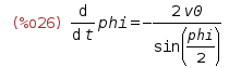

suits us. Now we substitute this angular velocity into the expression for the derivative of the covert of the unit vector of the rotation axis

du_mdt:ishow(subst(dphidt, du_mdt))$

and replace the derivatives of the remaining parameters of the quaternion

du_mdt:ishow(subst(v([m],[]), diff(p([m],[]),t), du_mdt))$

Well, we raise the indices, to obtain the derivative of the contravariant components of the unit vector

durdt:ishow(diff(u([],[r]),t) = contract(expand(rhs(du_mdt)*g([],[r,m]))))$

At the output, we have a complete set of expressions for performing the substitution.



Well, we execute them by opening the brackets along the path, forcing Maxima to reduce fractions if possible

Omega_1:ishow(subst(dphidt, Omega))$
Omega_1:ishow(expand(subst(du_mdt, Omega_1)))$
Omega_1:ishow(expand(subst(durdt, Omega_1)))$
Omega_1:ishow(expand(subst(u_i, Omega_1)))$
Omega_1:ishow(expand(subst(ur, Omega_1)))$

The result is already quite decent for itself,



but in the second term looms the vector product of the vector part of the quaternion itself, equal to zero. To SKA removed it, use the spell

Omega_2:ishow(canform(contract(expand(applyb1(Omega_1, lc_l, lc_u)))))$

Details of the construction of this command are described by me here . I recall only the point - to simplify the tensor expression according to the rules for working with convolutions of the Levi-Civita tensor. The spell removes the zero member.



Case for small - comb the trigonometry

Omega_3:ishow(trigsimp(Omega_2))$

and replace the remaining cosine with the scalar parameter of the quaternion

Omega_3:ishow(subst(lhs(Lambda0), rhs(Lambda0) , Omega_3))$

As a result, we have a rather compact expression. We



derive it in LaTeX

tentex(Omega_3);

Silent canform()indexes, numbered by the function, spoil the weather , but here we already use the handles to put the index names we need and at the same time return to the place the derivatives of the Rodrigue-Hamilton parameters



Expression (7) is the long-awaited expression of the angular velocity in terms of the Rodrigue-Hamilton parameters. As you can see, it is much more compact than the original expression written in the parameters of the final rotation. But this is not the only positive feature. Another nice feature will open to us when we get

3. Angular acceleration in the parameters of Rodrigue Hamilton

There are two ways to obtain angular acceleration. The first path, the simplest one, which for some reason I did not immediately get to, is simply to differentiate (7) in time. This is easily and quickly done manually. The second way I honestly crawled along was to get the formula in Maxima, simplifying the known expression of angular acceleration through the parameters of the final rotation



I will demonstrate both ways, only I will take the long way under the spoiler so that my dear reader does not lose the forests behind the trees.

So, we take the time derivative of (7)



The first term is zero, such are given up to the mutual destruction of members, and as a result, without much difficulty, we get





Suddenly, we observe a complete analogy with (7), only the second derivatives are here instead of the first derivatives. The coefficients for the derivatives are the same, which means that the angular velocity and angular acceleration are obtained from the corresponding derivatives of the Rodrigue-Hamilton parameters by multiplication by the same matrix (3 x 4). This, by the way, has determined the wide applicability of the quaternion approach in modeling the motion of spacecraft, and other objects that make free rotation in space.

Conclusion

The article went with a bias on the methods of working with tensor libraries Maxima. I can conclude that, even with the above assumptions, it is quite convenient to simplify tensor expressions in it.

And finally, we got the expressions of the angular velocity and angular acceleration through the Rodrigue-Hamilton orientation parameters convenient for modeling. And we were convinced that formulas (7) and (8) expressing them are not only compact, but also beautiful, in the sense that they use the same linear transformation of parameters to a quaternion to the components of the angular velocity and acceleration vectors. This approach greatly simplifies the organization of modeling programs, which we hope will be convinced of.

To date, we have come close to considering the dynamics of a free rigid body using a tensor apparatus. At the expense of the next article, I have an interesting idea, which I will try to implement and prepare high-quality material.

Thank you for attention!

To be continued...