Basics of programming on the SAS Base. Lesson 4: Creating SAS datasets
In the previous article, we explored how to read external raw data. And today we will get acquainted with the SET operator, which reads standard SAS data sets (SAS Data Set), learn how to create data slices, set up permanent attributes, and also learn some useful SAS functions. Again, I will try to present the material as simple as possible, using as many examples as possible.

 Suppose data is stored in EXCEL format in the directory C: \ workshop \ habrahabr . We import the spreadsheet, create a slice from it, create new calculated columns using SAS functions, and then break this data set into two.

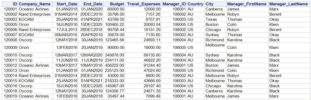
The excel file is stored in the directory specified above and has the following form:
File fragment:

Apply the PROC IMPORT procedure to convert a spreadsheet to a SAS dataset:
The option validvarname = V7 specifies the field names that are “correct” from the SAS point of view: all invalid characters are replaced with underscores. You can read about variable naming rules in Lesson 1.
We will set a filter immediately when reading an external file, for example, select only those observations in which the work completion date is not missed. Notice the syntax of the where parameter.
Let us consider in detail the step operators PROC IMPORT:
Datafile - defines the full path and name of the external file.
Dbms - determines the type of data to be imported.
Out — Identifies the output SAS dataset with a single or two-level SAS name (library name and dataset name).
Replace - overwrites an existing SAS dataset.
Getnames - Indicates whether PROC IMPORT generates SAS variable names from the data values in the first line in the input external file.
Run the PROC IMPORT step and examine the LOG:

Print the resulting SAS dataset:
The output of the PROC PRINT procedure is shown below:
Fragment:
You can also use the “Results” tab in the SAS UE and familiarize yourself with the imported SAS dataset.


Reading the SAS dataset is implemented in the DATA step using the SET statement :
Consider the general syntax of the SET statement:
If you do not specify a dataset in the SET statement, it reads the observations from the last created SAS dataset.
In the SET statement, you can specify multiple data sets, in this case, SAS Data Sets will be added one under the other (UNION equivalent in SQL).
Also, in the DATA step, there can be two SET statements, in this case the tables are joined by a common column. More information about the two SET operators can be found, for example, in this article .
The simplest code that creates a copy of the SAS dataset is as follows:
You can examine the SAS dataset descriptor using the PROC CONTENTS procedure ( see Lesson 2 ). In this lesson, we will print the descriptor component using the PROC DATASETS procedure :
Fragment of results:
Let's set a constant format for the Travel_Expenses and Budget variables:
Check the attributes of the SAS datasets:
All SAS functions can be explored in the SAS 9.4 Functions and CALL Routines Reference: Fifth Edition .
In addition, if there is no suitable function to perform a task, you can use the PROC FCMP procedure and create your own function.
In this lesson, we will explore the three functions of YRDIF, SUM and CATS.
To calculate the difference in dates in years, we will use the YRDIF function .
Let me remind you that the date in SAS format is the number of days since January 1, 1960 ( see Lesson 1 ). On the presented data, we need to calculate the execution time of the work:
Note that using the 3.1 format for the Lead_Time variable, we rounded the calculated values in the report (!) To 1 decimal. Operator format does not change the values in the SAS dataset!
Fragment of results:
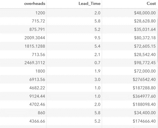
Next, we calculate the cost of work without travel expenses:
Fragment of results:
As part of our task, the cost of work, excluding travel expenses, we calculated without using a function. There are no missing values in our table, if one of the variables (Budget or Travel_Expenses) had a missing value, the result was “missing”.
For example:
Create a test dataset:
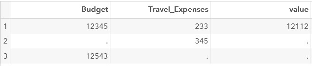
Calculate the difference of variables Budget Travel_Expenses
The result of this step:
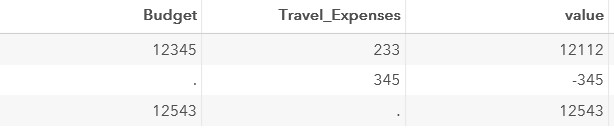
In order to get the correct result, you can use the SUM function .
This function falls into the category of descriptive statistics functions . The descriptive statistics functions ignore missing values.
Writing code through SUM:
In this case, the result of the step is as follows:
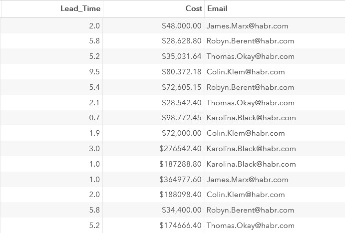
The third computed column is the manager's email address. It can be “assembled” from the Manager_FirstName, Manager_LastName columns and habr .com values .
You can use the CATS function to merge text values into one row .
Fragment of results:
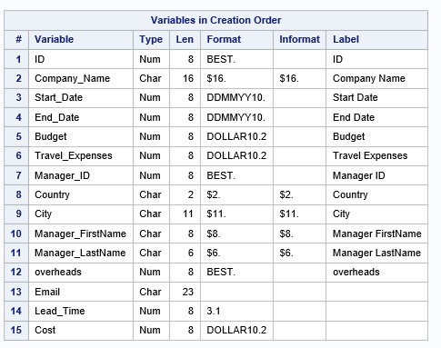
Examine the handle of the created dataset:
Handle fragment:

Notice the length of the Email variable. It is 200 bytes; this is the length returned by the default CATS function. If we examine the attributes of the variables Manager_FirstName and Manager_LastName, then we can make sure that the Email variable is 8 + 6 + the length of the string '@ habr.com', that is, 9 more bytes, total 23. Why should you pay attention to this? All missing characters achieve spaces, which affects the size of the data set and large data volumes will affect performance.
In order to set the length of the Email variable explicitly, you must use the LENGTH operator:
Handle Fragment
Create a detailed column based on the variable Lead_Time, taking into account the following conditions:
You can create a detailed column in different ways, for example, the simplest and most obvious option is to use conditional processing. It can be implemented using the following operators:
On large amounts of data it is more efficient to use the last two options.
Add a condition that selects only those observations in which the value of the Detail variable is not equal to 'above 5 years'. When using where as a filter, a syntax error will occur:
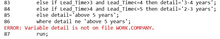
The where clause is not used for calculated columns. To select the variables we need, we need the selective IF operator. It cancels the output of the observation in the dataset being created:
Note also that the selective IF operator requires an arithmetic operator. We cannot write, for example, like this:
An error is displayed in the Log:

In the new SAS dataset, the variables Manager_FirstName and Manager_LastName should not be present. This requirement is implemented using the DROP parameter, you can also use the DROP operator.
We split the created SAS dataset into two according to the given condition
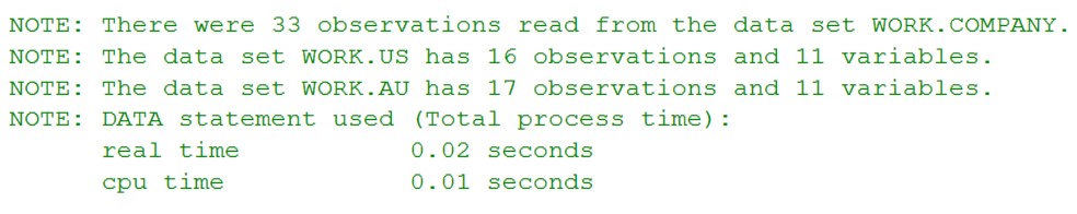
In one DATA step, you can create multiple SAS datasets. Let's create a separate data set for each country.
To check what values are in the Country column, you can, for example, use the PROC FREQ procedure .
This step counts the number of times a particular value from the Country variable is found in the SAS dataset specified in the data = parameter.
The result of this step will be as follows:

So, let's create two data sets in one DATA step using the OUTPUT operator and conditional processing:
Run the code and see the LOG:
This is a summary of reading and configuring SAS datasets. In the next article, we will introduce you to combining data sets using the MERGE and SET operators.
And as a PS, let me remind you the structure of our lessons on SAS BASE:
Articles that have already been published:
In the following articles I would like to highlight such issues as table association in SAS Base (merge, set), conditional processing, loops, SAS functions, creating custom formats, SAS Macro, PROC SQL.
 I would be happy to feedback in the comments! What other topics would you like to see in the articles?
Importing a spreadsheet and setting a filter
The excel file is stored in the directory specified above and has the following form:
File fragment:
Apply the PROC IMPORT procedure to convert a spreadsheet to a SAS dataset:
options validvarname=v7;
proc import datafile="C:\workshop\habrahabr\company.xlsx"
            dbms=xlsx
            out=company
            replace;
     		getnames=yes;
run;
The option validvarname = V7 specifies the field names that are “correct” from the SAS point of view: all invalid characters are replaced with underscores. You can read about variable naming rules in Lesson 1.
We will set a filter immediately when reading an external file, for example, select only those observations in which the work completion date is not missed. Notice the syntax of the where parameter.
options validvarname=v7;
proc import datafile="C:\workshop\habrahabr\company.xlsx"
            dbms=xlsx
            out=company (where=(End_Date notis missing))
            replace;
     		getnames=yes;
run;
Let us consider in detail the step operators PROC IMPORT:
Datafile - defines the full path and name of the external file.
Dbms - determines the type of data to be imported.
Out — Identifies the output SAS dataset with a single or two-level SAS name (library name and dataset name).
Replace - overwrites an existing SAS dataset.
Getnames - Indicates whether PROC IMPORT generates SAS variable names from the data values in the first line in the input external file.
Run the PROC IMPORT step and examine the LOG:
Print the resulting SAS dataset:
procprint data=work.company noobs;
run;
The output of the PROC PRINT procedure is shown below:
Fragment:
You can also use the “Results” tab in the SAS UE and familiarize yourself with the imported SAS dataset.
Reading SAS datasets
Reading the SAS dataset is implemented in the DATA step using the SET statement :
Consider the general syntax of the SET statement:
SET<SAS-data-set(s) <(data-set-options(s) )> > <options>;If you do not specify a dataset in the SET statement, it reads the observations from the last created SAS dataset.
In the SET statement, you can specify multiple data sets, in this case, SAS Data Sets will be added one under the other (UNION equivalent in SQL).
Also, in the DATA step, there can be two SET statements, in this case the tables are joined by a common column. More information about the two SET operators can be found, for example, in this article .
The simplest code that creates a copy of the SAS dataset is as follows:
data company1;
set company;
run;
Configuring a SAS Dataset Descriptor
You can examine the SAS dataset descriptor using the PROC CONTENTS procedure ( see Lesson 2 ). In this lesson, we will print the descriptor component using the PROC DATASETS procedure :
proc datasets library=work nolist;
contents data=company order=varnum;
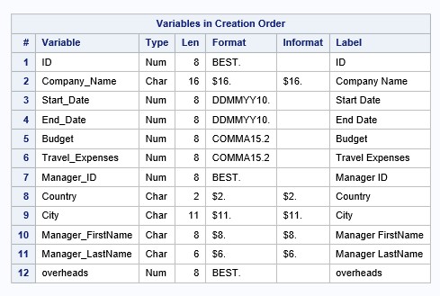
quit;Fragment of results:
Let's set a constant format for the Travel_Expenses and Budget variables:
data company;
set company;
format Travel_Expenses Budget dollar10.2;
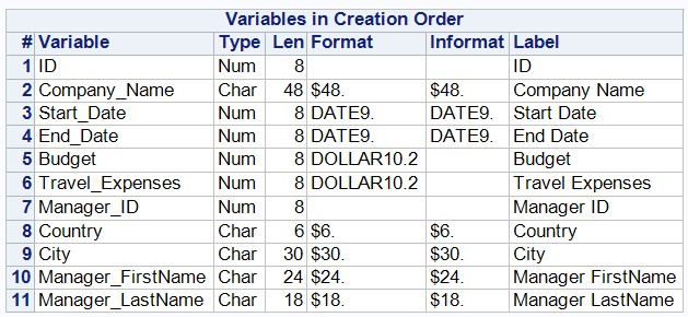
run;Check the attributes of the SAS datasets:
proc datasets library=work nolist;
contents data=company order=varnum;
quit;
Creating calculated columns
All SAS functions can be explored in the SAS 9.4 Functions and CALL Routines Reference: Fifth Edition .
In addition, if there is no suitable function to perform a task, you can use the PROC FCMP procedure and create your own function.
In this lesson, we will explore the three functions of YRDIF, SUM and CATS.
To calculate the difference in dates in years, we will use the YRDIF function .
Let me remind you that the date in SAS format is the number of days since January 1, 1960 ( see Lesson 1 ). On the presented data, we need to calculate the execution time of the work:
data company1;
setwork.company;
Lead_Time=yrdif(Start_Date, End_Date, 'actual');
format Travel_Expenses Budget dollar10.2 Lead_Time 3.1;
run;
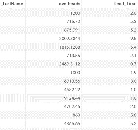
Note that using the 3.1 format for the Lead_Time variable, we rounded the calculated values in the report (!) To 1 decimal. Operator format does not change the values in the SAS dataset!
Fragment of results:
Next, we calculate the cost of work without travel expenses:
data company1;
setwork.company;
Lead_Time=yrdif(Start_Date, End_Date, 'actual');
Cost=Budget-Travel_Expenses;
formatCost Travel_Expenses Budget dollar10.2 Lead_Time 3.1;
run;
Fragment of results:
As part of our task, the cost of work, excluding travel expenses, we calculated without using a function. There are no missing values in our table, if one of the variables (Budget or Travel_Expenses) had a missing value, the result was “missing”.
For example:
Create a test dataset:
data test;inputBudgetTravel_Expenses;
datalines;
12345233
. 34512543 .
;
Calculate the difference of variables Budget Travel_Expenses
data test;
settest;
value=Budget-Travel_Expenses;
run;
The result of this step:
In order to get the correct result, you can use the SUM function .
This function falls into the category of descriptive statistics functions . The descriptive statistics functions ignore missing values.
Writing code through SUM:
data test;
set test;
value=sum(Budget,-Travel_Expenses);
run;
In this case, the result of the step is as follows:
The third computed column is the manager's email address. It can be “assembled” from the Manager_FirstName, Manager_LastName columns and habr .com values .
You can use the CATS function to merge text values into one row .
data company1;
setwork.company;
Lead_Time=yrdif(Start_Date, End_Date, 'actual');
Cost=Budget-Travel_Expenses;
Email=cats(Manager_FirstName, '.',Manager_LastName, '@habr.com');
formatCost Travel_Expenses Budget dollar10.2 Lead_Time 3.1;
run;
Fragment of results:
Examine the handle of the created dataset:
proc contents data=work.company1 varnum;run;Handle fragment:
Notice the length of the Email variable. It is 200 bytes; this is the length returned by the default CATS function. If we examine the attributes of the variables Manager_FirstName and Manager_LastName, then we can make sure that the Email variable is 8 + 6 + the length of the string '@ habr.com', that is, 9 more bytes, total 23. Why should you pay attention to this? All missing characters achieve spaces, which affects the size of the data set and large data volumes will affect performance.
In order to set the length of the Email variable explicitly, you must use the LENGTH operator:
data company1;
setwork.company;
length Email $23;
Lead_Time=yrdif(Start_Date, End_Date, 'actual');
Cost=Budget-Travel_Expenses;
Email=cats(Manager_FirstName, '.',Manager_LastName, '@habr.com');
formatCost Travel_Expenses Budget dollar10.2 Lead_Time 3.1;
run;
Handle Fragment
Create a detailed column based on the variable Lead_Time, taking into account the following conditions:
- If the value of the variable Lead_Time is less than 1, then the Detail column is less than 1 year.
- If the value of the variable Lead_Time is in the range from 1 to 2, including the borders, then the Detail column has a value of 1-2 years.
- If the value of the variable Lead_Time is in the range from 2 to 3, excluding 2, then the Detail column has a value of 2-3 years.
- If the value of the variable Lead_Time is in the range from 3 to 4, excluding 3, then the Detail column has a value of 3-4 years.
- If the value of the variable Lead_Time is in the range from 4 to 5, excluding 4, then the Detail column is 4-5 years.
- In all other cases, the Detail column is above 5 years.
You can create a detailed column in different ways, for example, the simplest and most obvious option is to use conditional processing. It can be implemented using the following operators:
- IF-THEN-ELSE
- ELSE IF
- SELECT-WHEN
On large amounts of data it is more efficient to use the last two options.
data company1;
setwork.company;
length Email $23;
Lead_Time=yrdif(Start_Date, End_Date, 'actual');
Cost=Budget-Travel_Expenses;
Email=cats(Manager_FirstName, '.',Manager_LastName, '@habr.com');
formatCost Travel_Expenses Budget dollar10.2 Lead_Time 3.1;
if Lead_Time<1then detail='less than a year';
elseif Lead_Time=>1and Lead_Time<=2then detail='1-2 years';
elseif Lead_Time>2and Lead_Time<=3then detail='2-3 years';
elseif Lead_Time>3and Lead_Time<=4then detail='3-4 years';
elseif Lead_Time>4and Lead_Time<=5then detail='4-5 years';
else detail='above 5 years';
run;
Add a condition that selects only those observations in which the value of the Detail variable is not equal to 'above 5 years'. When using where as a filter, a syntax error will occur:
The where clause is not used for calculated columns. To select the variables we need, we need the selective IF operator. It cancels the output of the observation in the dataset being created:
data company1;
setwork.company;
length Email $23;
Lead_Time=yrdif(Start_Date, End_Date, 'actual');
Cost=Budget-Travel_Expenses;
Email=cats(Manager_FirstName, '.',Manager_LastName, '@habr.com');
formatCost Travel_Expenses Budget dollar10.2 Lead_Time 3.1;
if Lead_Time<1then detail='less than a year';
elseif Lead_Time=>1and Lead_Time<=2then detail='1-2 years';
elseif Lead_Time>2and Lead_Time<=3then detail='2-3 years';
elseif Lead_Time>3and Lead_Time<=4then detail='3-4 years';
elseif Lead_Time>4and Lead_Time<=5then detail='2-3 years';
else detail='above 5 years';
if detail ne 'above 5 years';
run;
Note also that the selective IF operator requires an arithmetic operator. We cannot write, for example, like this:
if detail contains 'above 5 years';An error is displayed in the Log:
Configure the SAS dataset.
In the new SAS dataset, the variables Manager_FirstName and Manager_LastName should not be present. This requirement is implemented using the DROP parameter, you can also use the DROP operator.
data company1 (drop=Manager_FirstName Manager_LastName);
setwork.company;
length Email $23;
Lead_Time=yrdif(Start_Date, End_Date, 'actual');
Cost=Budget-Travel_Expenses;
Email=cats(Manager_FirstName, '.',Manager_LastName, '@habr.com');
formatCost Travel_Expenses Budget dollar10.2 Lead_Time 3.1;
if Lead_Time<1then detail='less than a year';
elseif Lead_Time=>1and Lead_Time<=2then detail='1-2 years';
elseif Lead_Time>2and Lead_Time<=3then detail='2-3 years';
elseif Lead_Time>3and Lead_Time<=4then detail='3-4 years';
elseif Lead_Time>4and Lead_Time<=5then detail='2-3 years';
else detail='above 5 years';
if detail ne 'above 5 years';
run;
We split the created SAS dataset into two according to the given condition
In one DATA step, you can create multiple SAS datasets. Let's create a separate data set for each country.
To check what values are in the Country column, you can, for example, use the PROC FREQ procedure .
proc freq data=company1;tableCountry /nocum nopercent;
run;
This step counts the number of times a particular value from the Country variable is found in the SAS dataset specified in the data = parameter.
The result of this step will be as follows:
So, let's create two data sets in one DATA step using the OUTPUT operator and conditional processing:
data US AU;
setwork.company1;
if Country='AU'then output AU;
if Country='US'then output US;
run;
Run the code and see the LOG:
This is a summary of reading and configuring SAS datasets. In the next article, we will introduce you to combining data sets using the MERGE and SET operators.
And as a PS, let me remind you the structure of our lessons on SAS BASE:
Articles that have already been published:
- Basics of programming on SAS BASE. Lesson 1.
- Basics of programming on SAS BASE. Lesson 2: Data Access
- Basics of programming on SAS BASE. Lesson 3. Reading text files.
- With the fourth lesson you just read.
In the following articles I would like to highlight such issues as table association in SAS Base (merge, set), conditional processing, loops, SAS functions, creating custom formats, SAS Macro, PROC SQL.
I would be happy to feedback in the comments! What other topics would you like to see in the articles?