DICOM Viewer from the inside. Functionality
Good afternoon, habrasociety. I would like to continue consideration of the implementation aspects of DICOM Viewer, and today we will focus on functionality.
So let's go.
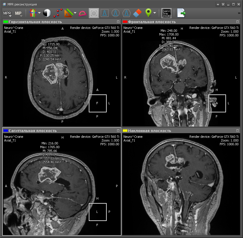
Multiplanar reconstruction allows you to create images from the original plane to the axial, frontal, sagittal or arbitrary plane. In order to build MPR, it is necessary to build a 3D volume model and “cut” it in the desired planes. As a rule, the best MPR quality is obtained with computed tomography (CT), because in the case of CT, you can create a 3D model with a resolution that is the same in all planes. Therefore, the output MPR is obtained with the same resolution as the original images obtained from CT. Although there are MRI with good resolution. Here is an example of a multi-planar reconstruction:
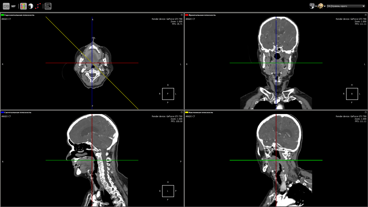
Green - axial plane (top left);
Red - the frontal plane (top right);
Blue - sagittal plane (bottom left);
Yellow - an arbitrary plane (bottom right).
The position of the lower right picture is determined by the yellow line in the side view (upper left). This is the image obtained by “cutting” the 3D model with an inclined plane. To obtain the density value at a specific point in the plane, trilinear interpolation is used.

The same as MPR, but instead of an arbitrary plane, you can take a curve, as shown in the figure. It is used, for example, in dentistry for a panoramic picture of teeth.
Each point on the curve defines the initial trace point, and the normal to the curve at this point corresponds to the direction of the Y axis in the two-dimensional image for this point. The X axis of the image corresponds to the curve itself. That is, at each point of the two-dimensional image, the direction of the X axis is the tangent to the curve at the corresponding point on the curve.
The values of minimum intensity show soft tissue. Whereas the values of maximum intensity correspond to the brightest areas of a three-dimensional object - these are either the most dense tissues or organs saturated with contrast medium. The minimum / average / maximum value of the intensity is taken in the range (as shown in the figure by dashed lines). The minimum value throughout the model will take air.
The MIP calculation algorithm is very simple: select a plane on a 3D model - let there be an XY plane. Then we go along the Z axis and select the maximum intensity value in a given range and display it on a 2D plane:
The image obtained by the projection of medium intensity is close to a conventional x-ray:
Some types of radiological studies do not give the desired effect without the use of a contrast agent, since they do not reflect certain types of tissues and organs. This is due to the fact that in the human body there are tissues whose density is approximately the same. To distinguish such tissues from each other, a contrast medium is used, which gives the blood a greater intensity. Also, a contrast agent is used to visualize blood vessels during angiography.
Angiography is a technique that allows you to visualize the blood flow systems (veins and blood vessels) of various organs. For this, a contrast medium is used, which is introduced into the organ under study, and an X-ray apparatus that creates images during the administration of the contrast medium. Thus, at the output of the apparatus, a set of images with a different degree of visualization of blood flows is obtained:
However, along with veins and vessels, tissues of other organs, such as the skull, are visible in the images. DSA (Digital subtraction angiography) mode allows you to visualize only blood flow without any other tissues. How it works? We take an image of a series in which blood flow has not yet been visualized with a contrast agent. As a rule, this is the first image of the series, the so-called mask:
Then we subtract this image from all the other images in the series. We get the following image:
In this image, blood flows are clearly visible and other tissues are practically invisible, which allows for a more accurate diagnosis.
The Clipping Box tool allows you to see bones and anatomical tissues in a section, as well as show internal organs from the inside. The tool is implemented at the render level, simply limiting the area of raytracing.
In the implementation, the area of raytracing is limited to planes with normals directed towards the cutoff. That is, the cube is represented by six planes.
The tool is similar to the previous one and allows you to delete a volume fragment under an arbitrary polygon:
Cutting should be understood as the vanishing of voxels in a 3D model that fall into the polygon.
There is also a tool “Scissors”, which allows you to remove parts of a 3D model according to the principle of connectivity. Implementation: when selecting an object, a cyclic search of nearby connected voxels takes place until all nearby voxels are viewed. Then all viewed voxels are deleted.
In 3D, you can measure organs at any angle, which is not possible for some cases in 2D.
In 3D mode, you can also use the polygon ruler:
PET-CT (eng. PET-CT) is a relatively new technology, which is a research method of nuclear medicine. It is a multimodal tomography method. The fourth dimension in this case is modality (PET and CT). It is intended mainly for the detection of cancerous tumors.
CT helps to get the anatomical structure of the human body:
and PET shows certain areas of concentration of a radioactive substance, which is directly related to the intensity of blood supply in this area.
PET obtains a picture of biochemical activity by detecting radioactive isotopes in the human body. A radioactive substance accumulates in organs saturated with blood. Then the radioactive substance undergoes positron beta decay. The resulting positrons are further annihilated with electrons from the surrounding tissue, as a result of which pairs of gamma rays are emitted, which are detected by the apparatus, and then a 3D image is built based on the received information.
The choice of a radioactive isotope determines the biological process that you want to track in the research process. The process can be metabolism, transport of substances, etc. The behavior of the process, in turn, is the key to the correct diagnosis of the disease. In the image above, a tumor is visible in the region of the liver.
But based on PET, it is difficult to understand in which part of the body is the area with the maximum concentration of the radioactive substance. When combining body geometry (CT) and areas saturated with blood with a high concentration of radioactive substance (PET), we obtain:
As a radioactive substance for PET, radioactive isotopes with different half-lives are used. Fluorine-18 (fluorodeoxyglucose) is used to form all kinds of malignant tumors, iodine-124 is used to diagnose thyroid cancer, gallium-68 is used to detect neuroendocrine tumors.
Functional Fusion forms a new series in which images of both modalities (and PET and CT) are combined. In the implementation, the images of both modalities are mixed, and then sorted along the Z axis (we assume that X and Y are the image axes). In fact, it turns out that the images in the series alternate (PET, CT, PET, CT ...). This series is later used for rendering 2D fusion and 3D fusion. In the case of 2D fusion, images are rendered in pairs (PET-CT) in ascending order of Z:
In this case, the CT image was first drawn, then PET.
3D fusion is implemented for a video card on CUDA. Both 3D models - PET and CT are drawn on the video card at the same time and it turns out a real multimodal fusion. On the processor, fusion also works, but it works in a slightly different way. The fact is that on the processor both models are represented in memory as separate octo trees. Therefore, when rendering, it is necessary to trace two trees and synchronize the passage of transparent voxels. And this would significantly reduce the speed of work. Therefore, it was decided to simply overlay the rendering result of one 3D model on top of another.
Cardiac CT technology is used to diagnose various cardiac abnormalities, including coronary heart disease, pulmonary embolism and other diseases.
4D Cardiac CT is 3D in time. Those. it turns out a small video, which we will call a loop, in which each frame will be a 3D object. The source data is a set of dicom images at once for all cinema loop frames. In order to convert a set of images into a cineloop, you must first group the original images into frames, and then create 3D for each frame. The construction of a 3D object at the frame level is the same as for any series of dicom images. We use heuristic sorting of images to group by frames, using the position of the image on the Z axis (assuming that X and Y are the image axis). We believe that after grouping by frames, the same number of images is obtained in each frame. Switching the frame actually comes down to switching the 3D model.
5D Fusion Pet - CardiacCT is a 4D Cardiac CT with the addition of fusion with PET as the fifth dimension. In the implementation, we first create two cinema loops: with CardiacCT and with PET. Then we make fuision of the corresponding frames of the film loop, which gives us a separate series. Then we build the 3D of the resulting series. It looks like this:
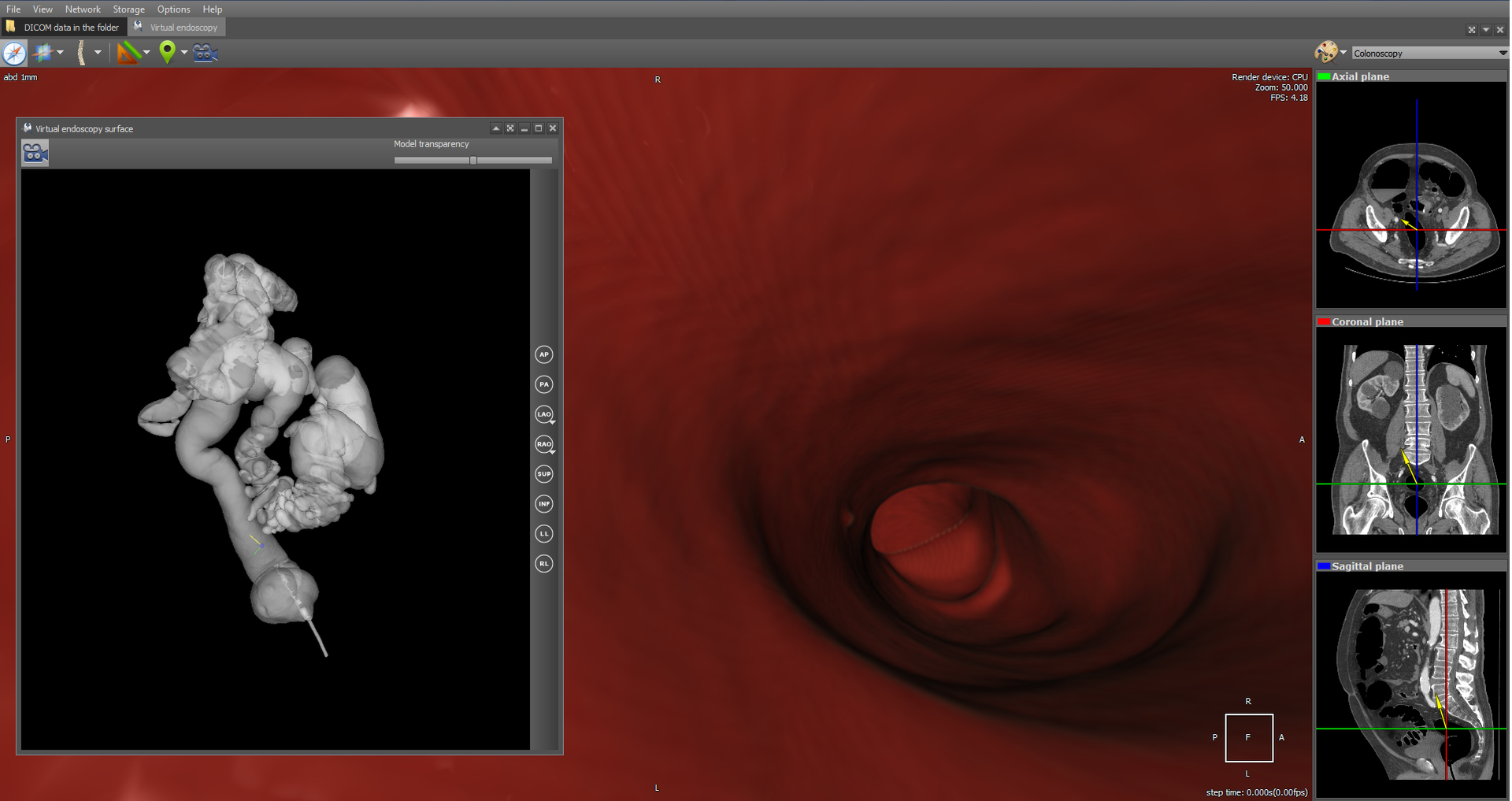
As an example of virtual endoscopy, we will consider virtual colonoscopy, since it is the most common type of virtual endoscopy. Virtual colonoscopy makes it possible to build a volumetric reconstruction of the abdominal region on the basis of CT data and make a diagnosis using this three-dimensional reconstruction. The viewer has a fly-through tool with MPR navigation:
which also allows you to automatically follow the anatomical structure. In particular, it allows you to view the intestinal region in automatic mode. Here's what it looks like:
The flight of the camera is a series of successive movements along the intestinal region. For each step, the vector of camera movement to the next part of the anatomical structure is calculated. The calculation is based on transparent voxels in the next part of the anatomical structure. In fact, a certain average voxel is calculated among the transparent ones. The initial displacement vector is specified by the camera vector. The Flight Camera tool uses an extremely perspective projection.
There is also functionality for automatic intestinal segmentation, i.e. functional for separating the intestinal region from the rest of the anatomy:
It is also possible to navigate through a segmented 3D model (the Show camera orientation button), which, by clicking on the 3D model, moves the camera to the corresponding position in the original anatomy.
Segmentation is implemented using the wave algorithm . It is believed that anatomy is closed in the sense that it does not contact with other organs and external space.
A separate module in the viewer implements reading data from Waveform and rendering them. DICOM ECG Waveform is a special format for storing electrocardiogram lead data, defined by the DICOM standard. These electrocardiograms represent twelve leads - 3 standard, 3 reinforced and 6 chest. The data of each lead is a sequence of measurements of electrical voltage on the surface of the body. In order to draw stresses, you need to know the vertical scale in mm / mV and the horizontal scale in mm / s:
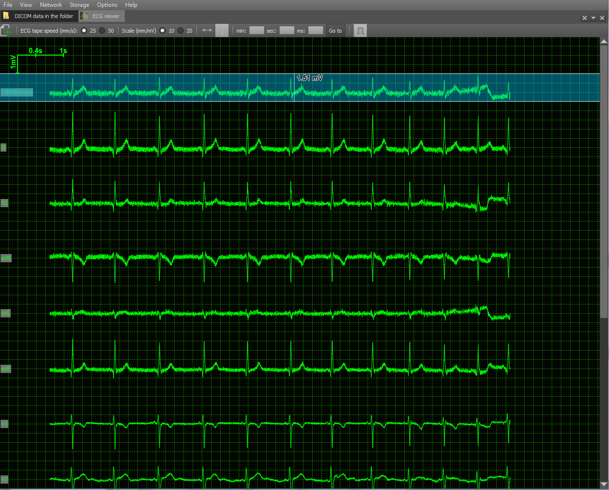
A grid is also rendered as auxiliary attributes for ease of distance measurement and scale in the upper left corner. Scale options are selected taking into account medical practice: vertically - 10 and 20 mm / mV, horizontally - 25 and 50 mm / sec. Also implemented tools for measuring distance horizontally and vertically.
DICOM-Viewer, among other things, is a full-fledged DICOM client. It is possible to search on a PACS server, obtain data from it, etc. The functions of the DICOM client are implemented using the DCMTK open library. Consider a typical use-case of a DICOM client using an example viewer. We search for stages on a remote PACS server:
When you select a stage, the series for the selected stage and the number of images in them are displayed below. At the top right is the PACS server on which the search will be performed. The search can be parameterized by specifying the search criteria: PID, date of examination, patient name, etc. Search on the client is performed by the C-FIND SCU team using the DCMTK library, which operates at one of the levels: STUDY, SERIES and IMAGE.
Further images of the selected series can be downloaded using the C-GET-SCU and C-MOVE-SCU commands. The DICOM protocol obliges the parties to the connection, i.e. client and server, agree in advance what types of data they are going to transmit through this connection. A data type is a combination of the values of the SOPClassUID and TransferSyntax parameters. SOPClassUID defines the type of operation to be performed through this connection. The most commonly used SOPClassUIDs: Verification SOP Class (server ping), Storage Service Class (image storage), Printer Sop Class (printing on a DICOM printer), CT Image Storage (CT image storage), MR Image Storage (image storage MRI) and others. TransferSyntax defines the format of the binary file. Popular TransferSyntax's: Little Endian Explicit, Big Endian Implicit, JPEG Lossless Nonhierarchical (Processes 14). That is, to transfer MRI images in Little Endian Implicit format, you need to add a pair of MR Image Storage - Little Endian Explicit to the connection.
The downloaded images are saved in the local storage and, when viewed again, are loaded from it, which allows to increase the viewer's productivity. Saved episodes are marked with a yellow icon in the upper left corner of the first episode image.
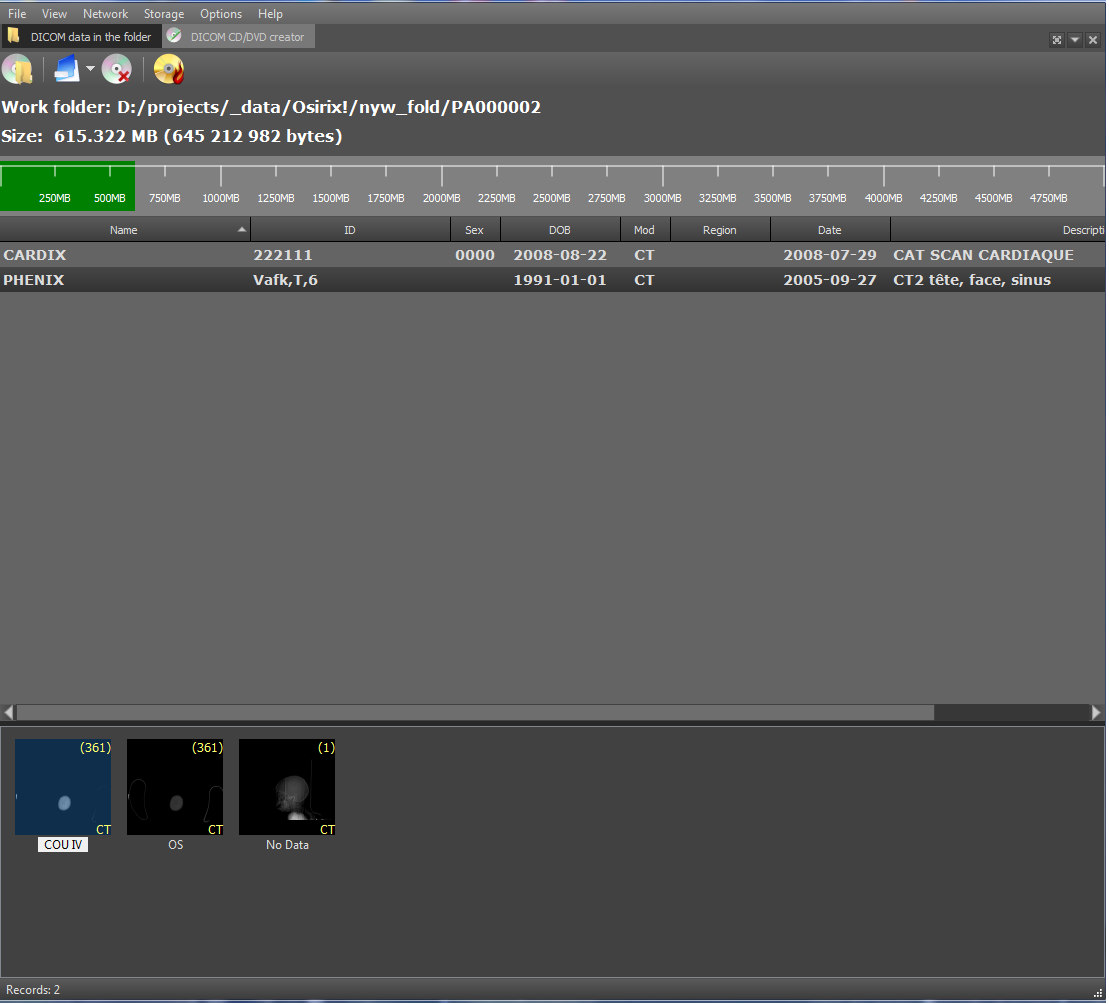
Also, DicomViewer, as a DICOM client, can burn research discs in the DICOMDIR format. The DICOMDIR format is implemented as a binary file that contains relative paths to all DICOM files that are written to disk. Implemented using the DCMTK library. When reading a disk, the paths to all files from DICOMDIR are read and then loaded. To add stages and series to DICOMDIR, the following interface was developed:
That's all I wanted to tell you about the functionality of DicomViewer. As always, feedback from qualified professionals is very welcome.
Viewer Link:
DICOM Viewer x86
DICOM Viewer x64
Data Examples:
MANIX - for general examples (MPR, 2D, 3D, etc.)
COLONIX - for virtual colonoscopy
FIVIX - 4D CARDIAC-CT
CEREBRIX - Fusion PET-CT
So let's go.
2D Toolkit
Multiplanar Reconstruction (MPR)
Multiplanar reconstruction allows you to create images from the original plane to the axial, frontal, sagittal or arbitrary plane. In order to build MPR, it is necessary to build a 3D volume model and “cut” it in the desired planes. As a rule, the best MPR quality is obtained with computed tomography (CT), because in the case of CT, you can create a 3D model with a resolution that is the same in all planes. Therefore, the output MPR is obtained with the same resolution as the original images obtained from CT. Although there are MRI with good resolution. Here is an example of a multi-planar reconstruction:
Green - axial plane (top left);
Red - the frontal plane (top right);
Blue - sagittal plane (bottom left);
Yellow - an arbitrary plane (bottom right).
The position of the lower right picture is determined by the yellow line in the side view (upper left). This is the image obtained by “cutting” the 3D model with an inclined plane. To obtain the density value at a specific point in the plane, trilinear interpolation is used.
Arbitrary Multiplanar Reconstruction (curved MPR)
The same as MPR, but instead of an arbitrary plane, you can take a curve, as shown in the figure. It is used, for example, in dentistry for a panoramic picture of teeth.
Each point on the curve defines the initial trace point, and the normal to the curve at this point corresponds to the direction of the Y axis in the two-dimensional image for this point. The X axis of the image corresponds to the curve itself. That is, at each point of the two-dimensional image, the direction of the X axis is the tangent to the curve at the corresponding point on the curve.
Minimum / Medium / Maximum Intensity Projection (MIP)
The values of minimum intensity show soft tissue. Whereas the values of maximum intensity correspond to the brightest areas of a three-dimensional object - these are either the most dense tissues or organs saturated with contrast medium. The minimum / average / maximum value of the intensity is taken in the range (as shown in the figure by dashed lines). The minimum value throughout the model will take air.
The MIP calculation algorithm is very simple: select a plane on a 3D model - let there be an XY plane. Then we go along the Z axis and select the maximum intensity value in a given range and display it on a 2D plane:
The image obtained by the projection of medium intensity is close to a conventional x-ray:
Some types of radiological studies do not give the desired effect without the use of a contrast agent, since they do not reflect certain types of tissues and organs. This is due to the fact that in the human body there are tissues whose density is approximately the same. To distinguish such tissues from each other, a contrast medium is used, which gives the blood a greater intensity. Also, a contrast agent is used to visualize blood vessels during angiography.
DSA mode for angiography
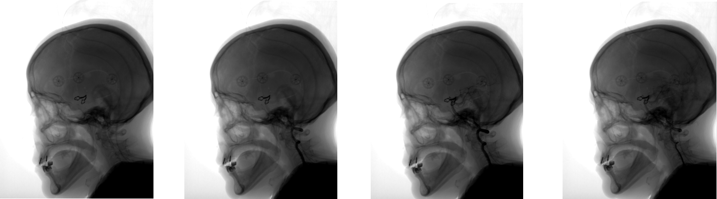
Angiography is a technique that allows you to visualize the blood flow systems (veins and blood vessels) of various organs. For this, a contrast medium is used, which is introduced into the organ under study, and an X-ray apparatus that creates images during the administration of the contrast medium. Thus, at the output of the apparatus, a set of images with a different degree of visualization of blood flows is obtained:
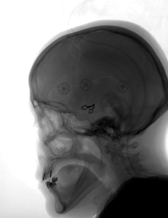
However, along with veins and vessels, tissues of other organs, such as the skull, are visible in the images. DSA (Digital subtraction angiography) mode allows you to visualize only blood flow without any other tissues. How it works? We take an image of a series in which blood flow has not yet been visualized with a contrast agent. As a rule, this is the first image of the series, the so-called mask:
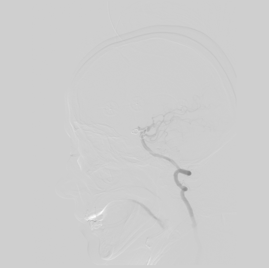
Then we subtract this image from all the other images in the series. We get the following image:
In this image, blood flows are clearly visible and other tissues are practically invisible, which allows for a more accurate diagnosis.
3D Toolkit
Clipping Box Tool
The Clipping Box tool allows you to see bones and anatomical tissues in a section, as well as show internal organs from the inside. The tool is implemented at the render level, simply limiting the area of raytracing.
In the implementation, the area of raytracing is limited to planes with normals directed towards the cutoff. That is, the cube is represented by six planes.
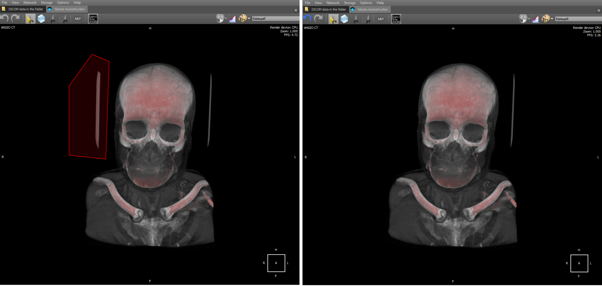
Volume Editing Toolkit - Polygon Cutting
The tool is similar to the previous one and allows you to delete a volume fragment under an arbitrary polygon:
Cutting should be understood as the vanishing of voxels in a 3D model that fall into the polygon.
There is also a tool “Scissors”, which allows you to remove parts of a 3D model according to the principle of connectivity. Implementation: when selecting an object, a cyclic search of nearby connected voxels takes place until all nearby voxels are viewed. Then all viewed voxels are deleted.
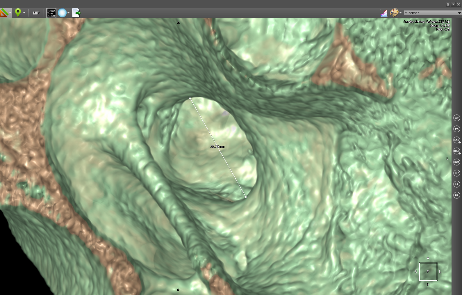
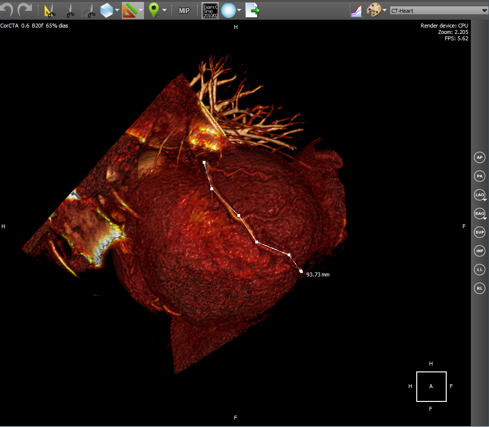
3D ruler
In 3D, you can measure organs at any angle, which is not possible for some cases in 2D.
In 3D mode, you can also use the polygon ruler:
Toolkit in 4D
Combining multiple tomographic series in 3D (Fusion PET-CT)
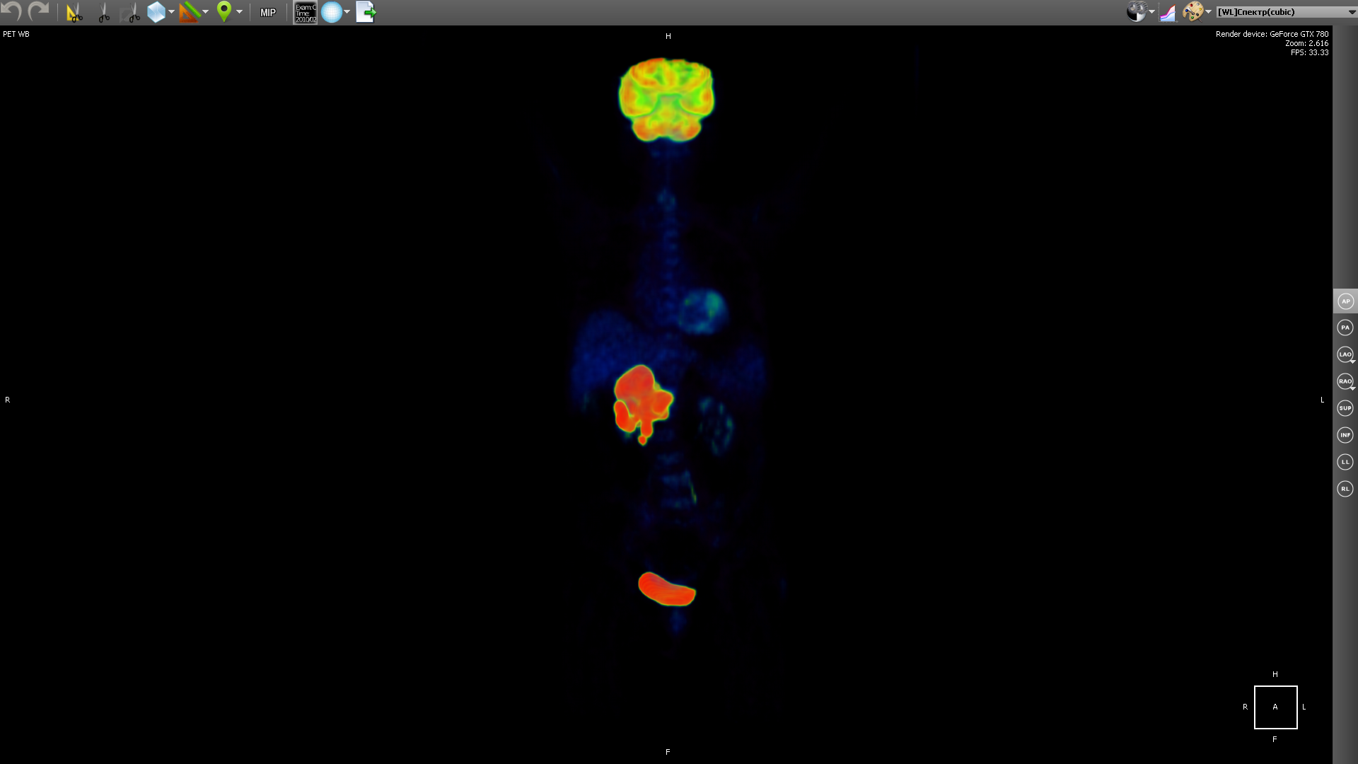
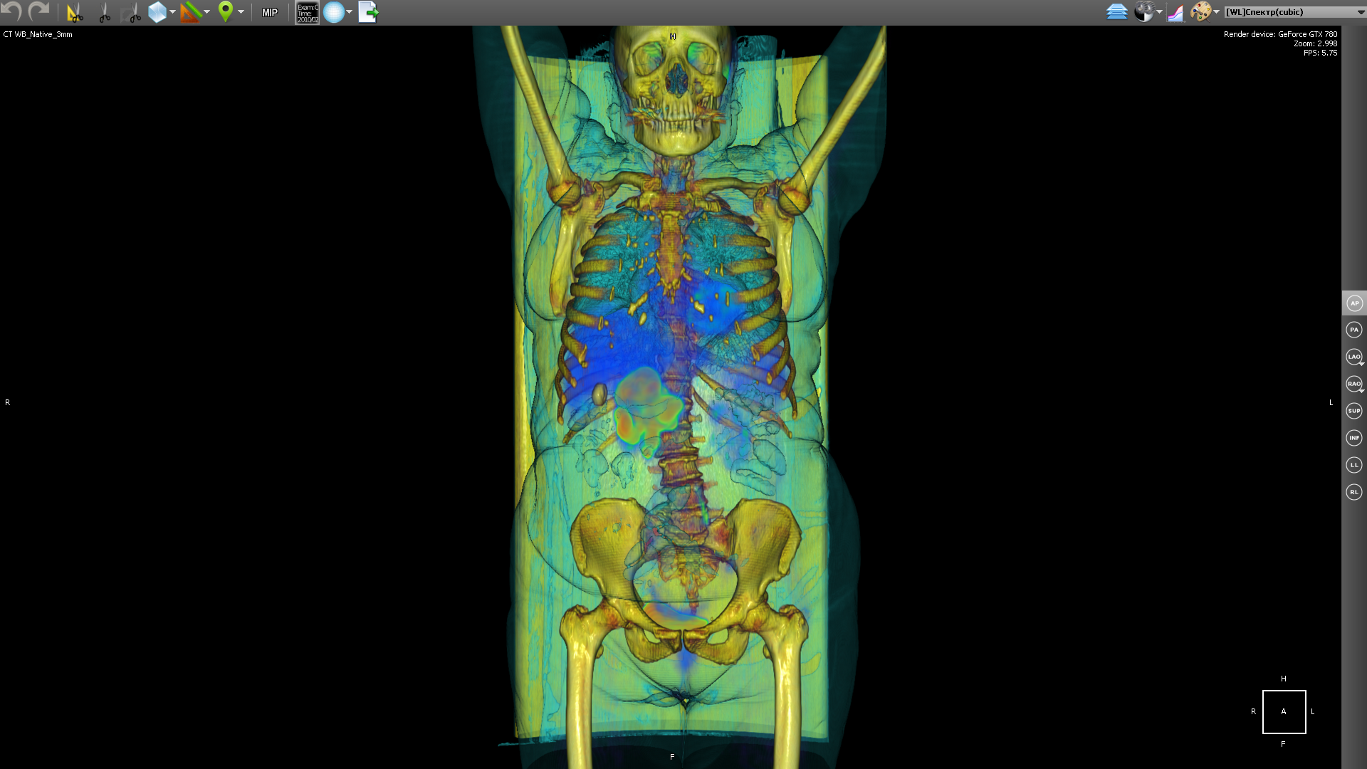
PET-CT (eng. PET-CT) is a relatively new technology, which is a research method of nuclear medicine. It is a multimodal tomography method. The fourth dimension in this case is modality (PET and CT). It is intended mainly for the detection of cancerous tumors.
CT helps to get the anatomical structure of the human body:
and PET shows certain areas of concentration of a radioactive substance, which is directly related to the intensity of blood supply in this area.
PET obtains a picture of biochemical activity by detecting radioactive isotopes in the human body. A radioactive substance accumulates in organs saturated with blood. Then the radioactive substance undergoes positron beta decay. The resulting positrons are further annihilated with electrons from the surrounding tissue, as a result of which pairs of gamma rays are emitted, which are detected by the apparatus, and then a 3D image is built based on the received information.
The choice of a radioactive isotope determines the biological process that you want to track in the research process. The process can be metabolism, transport of substances, etc. The behavior of the process, in turn, is the key to the correct diagnosis of the disease. In the image above, a tumor is visible in the region of the liver.
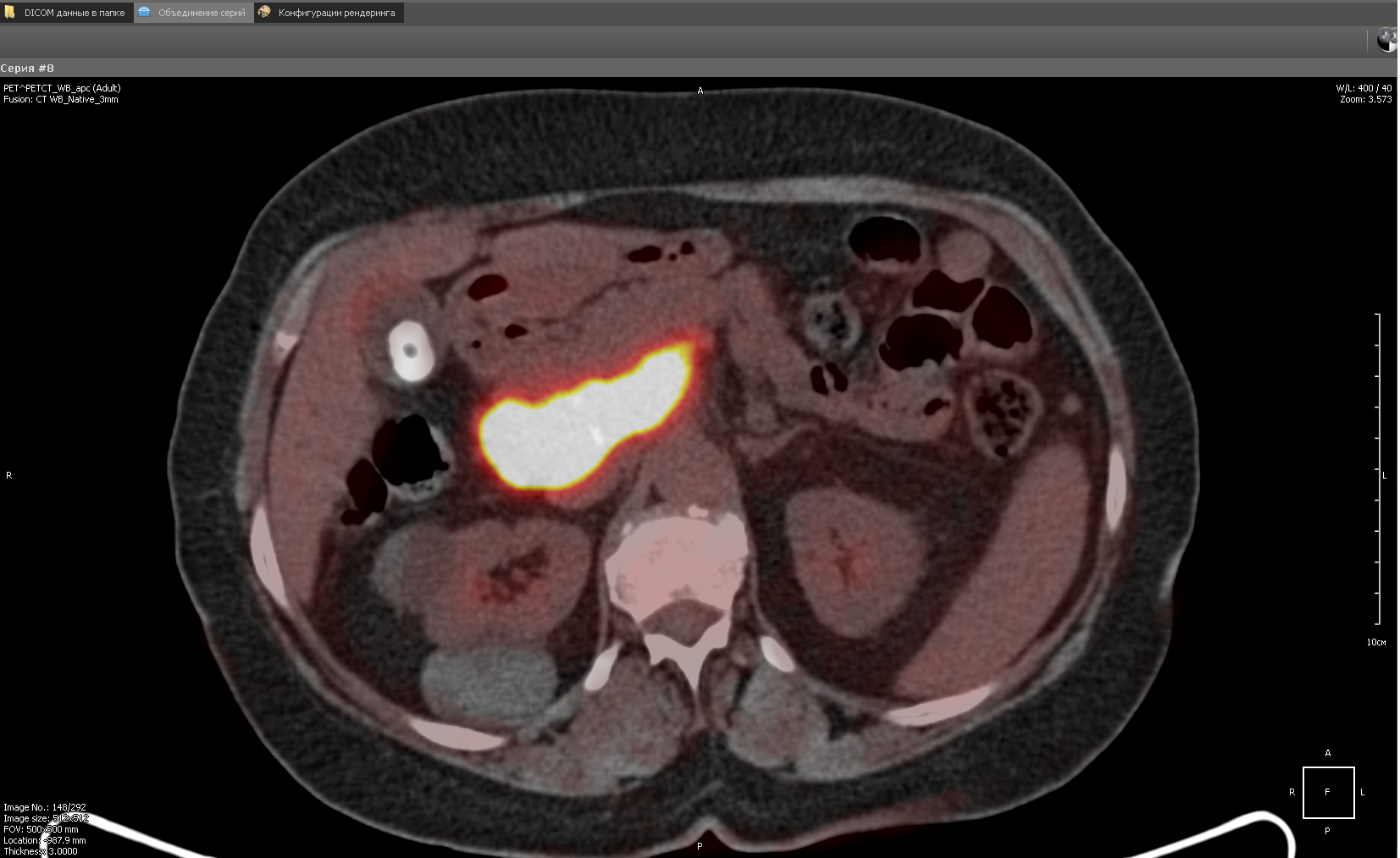
But based on PET, it is difficult to understand in which part of the body is the area with the maximum concentration of the radioactive substance. When combining body geometry (CT) and areas saturated with blood with a high concentration of radioactive substance (PET), we obtain:
As a radioactive substance for PET, radioactive isotopes with different half-lives are used. Fluorine-18 (fluorodeoxyglucose) is used to form all kinds of malignant tumors, iodine-124 is used to diagnose thyroid cancer, gallium-68 is used to detect neuroendocrine tumors.
Functional Fusion forms a new series in which images of both modalities (and PET and CT) are combined. In the implementation, the images of both modalities are mixed, and then sorted along the Z axis (we assume that X and Y are the image axes). In fact, it turns out that the images in the series alternate (PET, CT, PET, CT ...). This series is later used for rendering 2D fusion and 3D fusion. In the case of 2D fusion, images are rendered in pairs (PET-CT) in ascending order of Z:
In this case, the CT image was first drawn, then PET.
3D fusion is implemented for a video card on CUDA. Both 3D models - PET and CT are drawn on the video card at the same time and it turns out a real multimodal fusion. On the processor, fusion also works, but it works in a slightly different way. The fact is that on the processor both models are represented in memory as separate octo trees. Therefore, when rendering, it is necessary to trace two trees and synchronize the passage of transparent voxels. And this would significantly reduce the speed of work. Therefore, it was decided to simply overlay the rendering result of one 3D model on top of another.
4D CardiacCT
Cardiac CT technology is used to diagnose various cardiac abnormalities, including coronary heart disease, pulmonary embolism and other diseases.
4D Cardiac CT is 3D in time. Those. it turns out a small video, which we will call a loop, in which each frame will be a 3D object. The source data is a set of dicom images at once for all cinema loop frames. In order to convert a set of images into a cineloop, you must first group the original images into frames, and then create 3D for each frame. The construction of a 3D object at the frame level is the same as for any series of dicom images. We use heuristic sorting of images to group by frames, using the position of the image on the Z axis (assuming that X and Y are the image axis). We believe that after grouping by frames, the same number of images is obtained in each frame. Switching the frame actually comes down to switching the 3D model.
5D Fusion Pet - CardiacCT
5D Fusion Pet - CardiacCT is a 4D Cardiac CT with the addition of fusion with PET as the fifth dimension. In the implementation, we first create two cinema loops: with CardiacCT and with PET. Then we make fuision of the corresponding frames of the film loop, which gives us a separate series. Then we build the 3D of the resulting series. It looks like this:
Virtual endoscopy
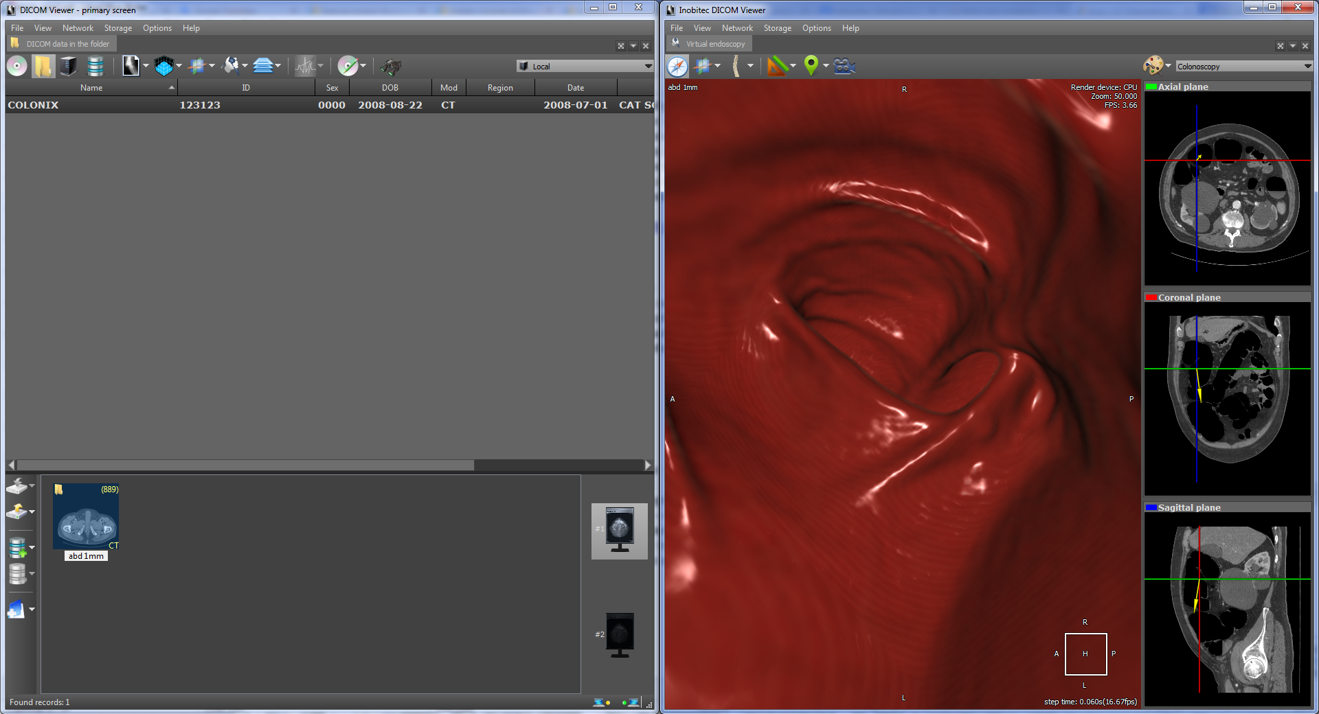
As an example of virtual endoscopy, we will consider virtual colonoscopy, since it is the most common type of virtual endoscopy. Virtual colonoscopy makes it possible to build a volumetric reconstruction of the abdominal region on the basis of CT data and make a diagnosis using this three-dimensional reconstruction. The viewer has a fly-through tool with MPR navigation:
which also allows you to automatically follow the anatomical structure. In particular, it allows you to view the intestinal region in automatic mode. Here's what it looks like:
The flight of the camera is a series of successive movements along the intestinal region. For each step, the vector of camera movement to the next part of the anatomical structure is calculated. The calculation is based on transparent voxels in the next part of the anatomical structure. In fact, a certain average voxel is calculated among the transparent ones. The initial displacement vector is specified by the camera vector. The Flight Camera tool uses an extremely perspective projection.
There is also functionality for automatic intestinal segmentation, i.e. functional for separating the intestinal region from the rest of the anatomy:
It is also possible to navigate through a segmented 3D model (the Show camera orientation button), which, by clicking on the 3D model, moves the camera to the corresponding position in the original anatomy.
Segmentation is implemented using the wave algorithm . It is believed that anatomy is closed in the sense that it does not contact with other organs and external space.
ECG Viewer (Waveform)
A separate module in the viewer implements reading data from Waveform and rendering them. DICOM ECG Waveform is a special format for storing electrocardiogram lead data, defined by the DICOM standard. These electrocardiograms represent twelve leads - 3 standard, 3 reinforced and 6 chest. The data of each lead is a sequence of measurements of electrical voltage on the surface of the body. In order to draw stresses, you need to know the vertical scale in mm / mV and the horizontal scale in mm / s:
A grid is also rendered as auxiliary attributes for ease of distance measurement and scale in the upper left corner. Scale options are selected taking into account medical practice: vertically - 10 and 20 mm / mV, horizontally - 25 and 50 mm / sec. Also implemented tools for measuring distance horizontally and vertically.
DICOM Viewer as a DICOM Client
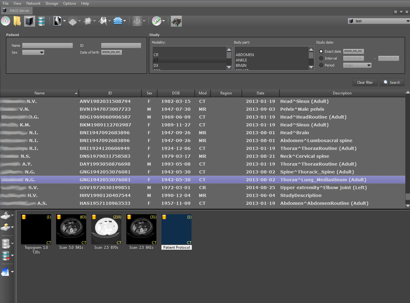
DICOM-Viewer, among other things, is a full-fledged DICOM client. It is possible to search on a PACS server, obtain data from it, etc. The functions of the DICOM client are implemented using the DCMTK open library. Consider a typical use-case of a DICOM client using an example viewer. We search for stages on a remote PACS server:
When you select a stage, the series for the selected stage and the number of images in them are displayed below. At the top right is the PACS server on which the search will be performed. The search can be parameterized by specifying the search criteria: PID, date of examination, patient name, etc. Search on the client is performed by the C-FIND SCU team using the DCMTK library, which operates at one of the levels: STUDY, SERIES and IMAGE.
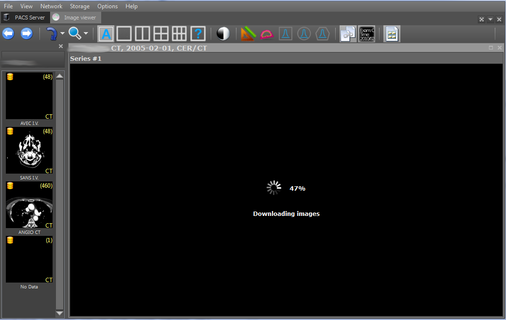
Further images of the selected series can be downloaded using the C-GET-SCU and C-MOVE-SCU commands. The DICOM protocol obliges the parties to the connection, i.e. client and server, agree in advance what types of data they are going to transmit through this connection. A data type is a combination of the values of the SOPClassUID and TransferSyntax parameters. SOPClassUID defines the type of operation to be performed through this connection. The most commonly used SOPClassUIDs: Verification SOP Class (server ping), Storage Service Class (image storage), Printer Sop Class (printing on a DICOM printer), CT Image Storage (CT image storage), MR Image Storage (image storage MRI) and others. TransferSyntax defines the format of the binary file. Popular TransferSyntax's: Little Endian Explicit, Big Endian Implicit, JPEG Lossless Nonhierarchical (Processes 14). That is, to transfer MRI images in Little Endian Implicit format, you need to add a pair of MR Image Storage - Little Endian Explicit to the connection.
The downloaded images are saved in the local storage and, when viewed again, are loaded from it, which allows to increase the viewer's productivity. Saved episodes are marked with a yellow icon in the upper left corner of the first episode image.
Also, DicomViewer, as a DICOM client, can burn research discs in the DICOMDIR format. The DICOMDIR format is implemented as a binary file that contains relative paths to all DICOM files that are written to disk. Implemented using the DCMTK library. When reading a disk, the paths to all files from DICOMDIR are read and then loaded. To add stages and series to DICOMDIR, the following interface was developed:
That's all I wanted to tell you about the functionality of DicomViewer. As always, feedback from qualified professionals is very welcome.
Viewer Link:
DICOM Viewer x86
DICOM Viewer x64
Data Examples:
MANIX - for general examples (MPR, 2D, 3D, etc.)
COLONIX - for virtual colonoscopy
FIVIX - 4D CARDIAC-CT
CEREBRIX - Fusion PET-CT