The principle of least action. Part 2

The last time we looked briefly at one of the most remarkable physical principles - the principle of least action, and stopped for example, which would seem to contradict it. In this article we will deal with this principle in a little more detail and see what happens in this example.

This time we need a little more math. However, I will again try to explain the main part of the article at an elementary level. I will highlight slightly more rigorous and difficult points, they can be skipped without prejudice to the basic understanding of the article.

Border conditions

We begin with the simplest object - a ball that moves freely in space, on which no forces act. Such a ball, as you know, moves uniformly and straightforwardly. For simplicity, suppose it moves along the axis$$:

To accurately describe its movement, as a rule, initial conditions are specified. For example, it is specified that at the initial moment of time$$ the ball was at the point $$ with coordinate $$ and had speed $$. By setting the initial conditions in this form, we uniquely determine the further movement of the ball - it will move at a constant speed, and its position at the moment of time$$ will be equal to the starting position plus the speed multiplied by the past tense: $$. This way of setting the initial conditions is very natural and intuitively familiar. We set all the necessary information about the motion of the ball at the initial moment of time, and then its motion is determined by the laws of Newton.

However, this is not the only way to specify the movement of the ball. Another alternative is to position the ball at two different points in time.$$ and $$. Those. set that:

1) at the moment of time$$ the ball was at the point $$ (with coordinate $$);
2) at the moment of time$$ the ball was at the point $$ (with coordinate $$).

The expression "was at the point$$"Does not mean that the ball rested at a point $$. At the moment of time$$ he could fly through the point $$. It means that his position at the moment of time$$ match point $$. The same applies to the point$$.

These two conditions also uniquely determine the motion of the ball. His movement is easy to calculate. To satisfy both conditions, the speed of the ball obviously must be$$. The position of the ball at a time$$ will again be equal to the starting position plus the speed multiplied by the past tense:

$$

Note that under the conditions of the problem we did not need to set the initial velocity. It is uniquely determined from conditions 1) and 2).

Setting conditions in the second way looks unusual. It may not be clear why it may even be necessary to ask them in this form. However, in principle, the smallest action uses the conditions in the form of 1) and 2), and not in the form of setting the initial position and initial velocity.

Trajectory with the least action

Now let's digress from the real free movement of the ball and consider the following purely mathematical problem. Suppose we have a ball, which we can manually move in any way we like. At the same time, we need to fulfill conditions 1) and 2). Those. in the interval between$$ and $$ we have to move it from point $$ exactly $$. This can be done in completely different ways. Each such method we will call the trajectory of the ball and it can be described by a function of the ball's position from time to time.$$. Let us postpone several such trajectories on the graph of the ball's position versus time:

For example, we can move a ball with the same speed equal to $$(green trajectory). Or we can keep it at half time$$and then double speed move to a point $$(blue trajectory). You can first move it to the opposite of$$ side and then move to $$(brown trajectory). You can move it back and forth (red path). In general, you can move it as you please, if only conditions 1) and 2) are met.

For each such trajectory, we can match the number. In our example, i.e. in the absence of any forces acting on the ball, this number is equal to the total accumulated kinetic energy for the entire time of its movement in the time interval between$$ and $$ and called action.

In this case, the word “accumulated” kinetic energy does not accurately convey the meaning. In reality, kinetic energy does not accumulate anywhere; accumulation is used only to calculate the action for the trajectory. In mathematics for such accumulation there is a very good concept - the integral:

$$

An action is usually denoted by a letter. $$. Symbol$$means kinetic energy. This integral means that the action is equal to the accumulated kinetic energy of the ball over a period of time from$$ before $$.

As an example, let's take a ball with a mass of 1 kg., Set some boundary conditions and calculate the action for two different trajectories. Let dot$$ located at a distance of 1 meter from the point $$and time $$ away from time $$for 1 second. Those. we have to move the ball, which at the initial moment of time was at$$, in one second at a distance of 1 m. along the axis $$.

In the first example (green path) we moved the ball evenly, i.e. with the same speed, which obviously should be equal to:$$m / s The kinetic energy of the ball at each time instant is equal to:$$ = 1/2 J. In one second 1/2 J will accumulate. $$with kinetic energy. Those. Act for such a trajectory is:$$ J $$with.

Now let's not move the ball right from the point.$$ exactly $$, and hold it for half a second at $$and then, for the remaining time, move it evenly to a point. $$. In the first half second the ball is at rest and its kinetic energy is zero. Therefore, the contribution to the action of this part of the trajectory is also zero. The second half-second we carry the ball with double speed:$$m / s The kinetic energy will be equal to$$= 2 J. The contribution of this time interval to the action will be equal to 2 J multiplied by half a second, i.e. 1 j$$with. Therefore, the general action for such a trajectory is equal to$$ J $$with.

Similarly, any other trajectory with the given boundary conditions 1) and 2) corresponds to a number equal to the action for this trajectory. Among all such trajectories there is a trajectory that has the least action. It can be proved that this trajectory is a green trajectory, i.e. uniform ball movement. For any other trajectory, however cunning it may be, the action will be greater than 1/2.

In mathematics, such a comparison for each function of a certain number is called a functional. Quite often in physics and mathematics, problems arise like ours, i.e. to find a function for which the value of a certain functional is minimal. For example, one of the tasks of great historical importance for the development of mathematics is the problem of bachistochrone. Those. finding a curve along which the ball rolls down the fastest. Again, each curve can be represented by the function h (x), and each function is assigned a number, in this case, the time it takes for the ball to roll. Again, the problem is reduced to finding a function for which the value of the functional is minimal. The area of ​​mathematics that deals with such tasks is called calculus of variations.

Principle of least action

In the examples analyzed above, we have two special trajectories obtained in two different ways.

The first trajectory is obtained from the laws of physics and corresponds to the real trajectory of a free ball, on which no forces act, and for which the boundary conditions are given in the form 1) and 2).

The second trajectory is obtained from the mathematical problem of finding a trajectory with given boundary conditions 1) and 2), for which the action is minimal.

The principle of least action states that these two trajectories must coincide. In other words, if it is known that the ball moved in such a way that the boundary conditions 1) and 2) were satisfied, then it necessarily moved along a trajectory for which the action is minimal compared to any other trajectory with the same boundary conditions.

It would be a coincidence. It is not enough tasks in which uniform trajectories and straight lines appear. However, the principle of least action turns out to be a very general principle, which is also valid in other situations, for example, for the ball to move in a uniform field of gravity. For this, it is only necessary to replace the kinetic energy with the difference between the kinetic and potential energy. This difference is called the Lagrangian or the Lagrange function and the action now becomes equal to the total accumulated Lagrangian. In fact, the Lagrange function contains all the necessary information about the dynamic properties of the system.

If we run the ball in a uniform field of gravity so that it flew past the point$$ at time $$ and flew to the point $$ at time $$, he, according to Newton's laws, will fly in a parabola. It is this parabola that coincides with the trajectories for which the action will be minimal.

Thus, for a body moving in a potential field, for example, in the gravitational field of the Earth, the Lagrange function is equal to: $$. Kinetic energy$$depends on the speed of the body, and the potential - on its position, i.e. coordinates$$. In analytical mechanics, the entire set of coordinates that determine the position of a system is usually denoted by a single letter.$$. For a ball moving freely in a gravity field$$ mean coordinates $$, $$ and $$.

To indicate the rate of change of a quantity, in physics it is often very easy to put a dot over this quantity. For example,$$ denotes the rate of change of the coordinate $$or, in other words, the speed of the body in the direction $$. Using these conventions, the speed of our ball in analytical mechanics is denoted as$$. Those.$$ means speed components $$.

Since the Lagrange function depends on speed and coordinates, it can also explicitly depend on time (obviously depends on time means that$$ at different points in time is different, at the same speeds and positions of the ball), the action in general form is written as

$$

Not always the minimum

However, at the end of the previous part, we looked at an example where the principle of least action clearly does not work. To do this, we again took a free ball, on which no forces act, and placed a spring wall next to it.
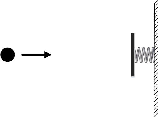
The boundary conditions we set are such that the points $$ and $$match up. Those. and at the time$$ and at the time $$ the ball must be at the same point $$. One of the possible trajectories will be the standing of the ball in place. Those. the entire time span$$ and $$ he will stand at a point $$. The kinetic and potential energy in this case will be equal to zero, therefore the action for such a trajectory will also be equal to zero.

Strictly speaking, the potential energy can be taken equal not to zero, but to any number, since the difference between the potential energy at different points in space is important. However, a change in the value of potential energy does not affect the finding of a trajectory with minimal action. It is just that for all trajectories the value of the action will change by the same number, and the trajectory with the minimum action will remain the trajectory with the minimum action. For convenience, for our ball, we choose the potential energy equal to zero.

Another possible physical trajectory with the same boundary conditions is the trajectory at which the ball first flies to the right, passing the point $$ at time $$. Then he collides with the spring, squeezes it, the spring, straightening, pushes the ball back, and again it flies past the point$$. You can choose the speed of the ball so that it, bounced off the wall, flying point$$ exactly at the moment $$. The action with such a trajectory will be basically equal to the accumulated kinetic energy during the flight between the point$$and wall and back. There will be some period of time when the ball will compress the spring and its potential energy will increase, and during this period of time the potential energy will make a negative contribution to the action. But such a period of time will not be very large and will not significantly reduce the effect.



The figure shows both physically possible trajectories of the ball. The green path corresponds to the resting ball, while the blue corresponds to the ball that bounced off the spring wall.

However, only one of them has a minimal effect, namely the first! The second trajectory has more action. It turns out that in this problem there are two physically possible trajectories and only one with minimal action. Those. in this case, the principle of least action does not work.

Stationary points

To understand what this is all about, let's digress from the principle of least action for the time being and deal with ordinary functions. Let's take some function$$ and draw its schedule:

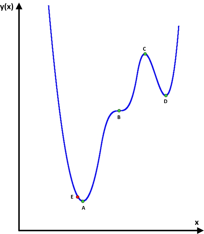
On the chart, I marked four green points in green. What is common to these points? Imagine that a function graph is a real slide on which a ball can roll. The four points marked are special in that if you set the ball exactly at a given point, it will not roll away anywhere. In all other points, for example, point E, he will not be able to stand still and will begin to roll down. Such points are called stationary. Finding such points is a useful task, since any maximum or minimum of a function, if it does not have sharp breaks, must necessarily be a stationary point.

If it is more accurate to classify these points, then point A is the absolute minimum of the function, i.e. its value is less than any other function value. Point B is neither a maximum nor a minimum and is called a saddle point. Point C is called a local maximum, i.e. its value is greater than at neighboring points of the function. And point D is a local minimum, i.e. its value is less than at neighboring points of the function.

The search for such points is engaged in the section of mathematics, called mathematical analysis. Otherwise, it is sometimes called the analysis of infinitely small, since it can work with infinitesimally small quantities. From the point of view of mathematical analysis, stationary points have one special property due to which they are found. To understand what this property is, we need to understand how a function looks at very small distances from these points. To do this, we take a microscope and look at it at our points. The figure shows what the function looks like in the vicinity of different points at different magnifications.

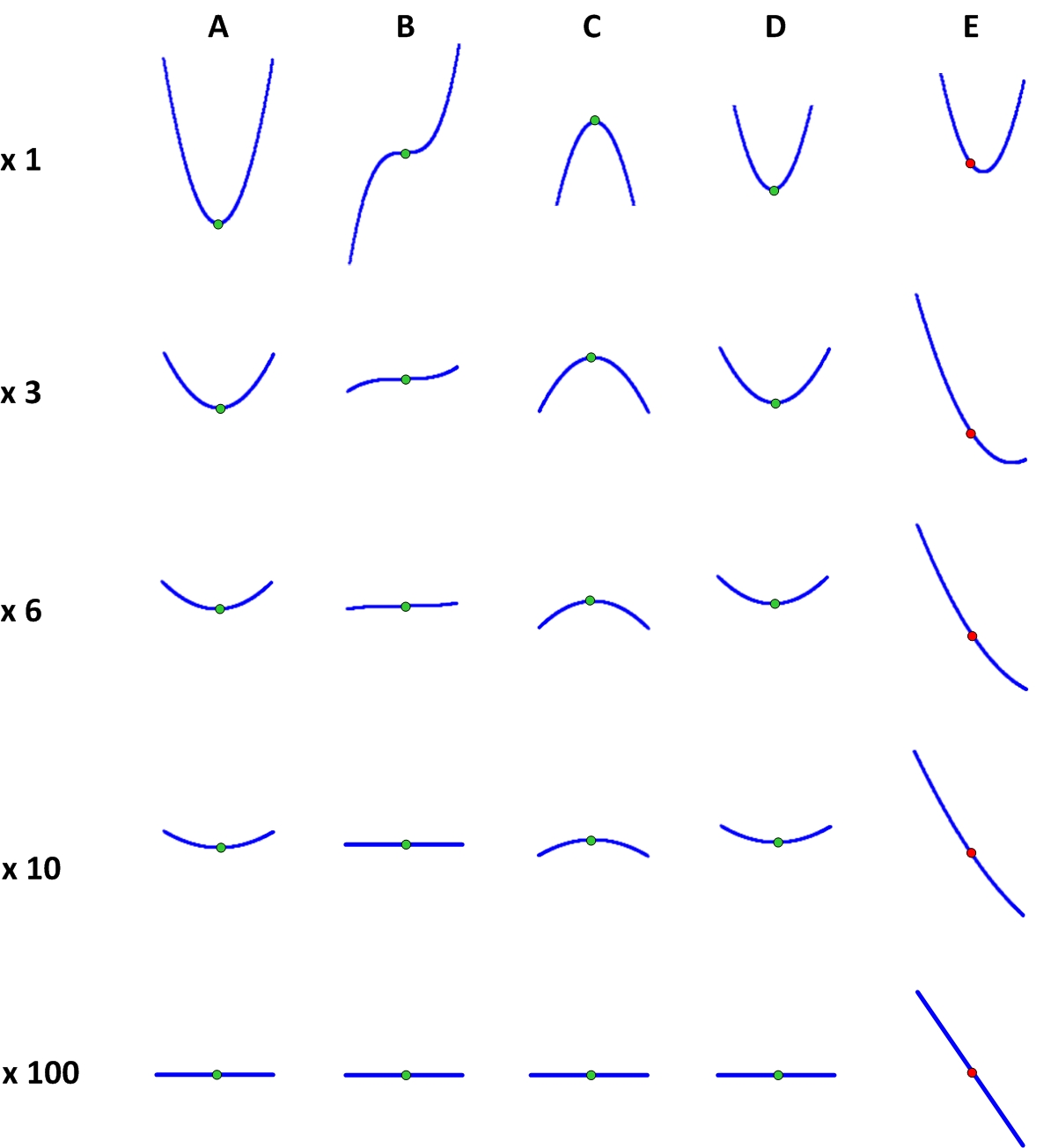
It can be seen that with a very large magnification (that is, with very small deviations of x), the stationary points look exactly the same and are very different from the non-stationary point. It is easy to understand what this difference is - the graph of the function at a stationary point with increasing becomes a strictly horizontal line, and in a non-stationary one it is an inclined one. That is why the ball installed at a stationary point will not roll.

The horizontality of a function at a stationary point can be expressed differently: the function at a stationary point remains almost unchanged with a very small change in its argument$$, even in comparison with the argument itself. The function is in a non-stationary point with a small change$$ changes in proportion to change $$. And the greater the angle of inclination of the function, the more the function changes when changing$$. In fact, when zoomed, the function becomes more and more like the tangent to the graph at the point in question.

In strict mathematical language, the expression “the function practically does not change at the point $$ with very little change $$"Means that the relationship of changing a function and changing its argument $$ tends to 0 when $$ tending to 0:

$\$\$\; display\; \$\$\; \backslash \; lim\_\; \{∆x\; \backslash \; to\; 0\}\; \backslash \; frac\; \{∆y\; (x\_0)\}\; \{∆x\}\; =\; \backslash \; lim\_\; \{x\; \backslash \; to\; 0\}\; \backslash \; frac\; \{y\; (x\_0\; +\; ∆x)\; -y\; (x\_0)\; \}\; \{∆x\}\; =\; 0\; \$\$\; display\; \$\$$

For a nonstationary point, this ratio tends to a nonzero number, which is equal to the tangent of the angle of inclination of the function at that point. The same number is called the derivative of the function at a given point. The derivative of a function shows how quickly a function changes around a given point with a small change in its argument.$$. Thus, the stationary points are the points at which the derivative of the function is 0.

Stationary trajectories

By analogy with stationary points, one can introduce the concept of stationary trajectories. Recall that for each trajectory we have a certain value of the action, i.e. some number. Then such a trajectory can be found that for trajectories close to it with the same boundary conditions, the corresponding action values ​​will hardly differ from the action for the stationary trajectory itself. Such a trajectory is called stationary. In other words, any trajectory close to stationary will have an action value that differs very little from that for this stationary trajectory.

Again, in mathematical language, "slightly different" has the following exact meaning. Suppose that we have defined the functionality$$ for functions with the required boundary conditions 1) and 2), i.e. $$ and $$. Assume that the trajectory$$- stationary.

We can take any other function.$$, such that at the ends it takes zero values, i.e. $$ = $$ = 0. Also take the variable $$which we will do less and less. Of these two functions and variable$$ we can make up the third function $$which will also satisfy the boundary conditions $$ and $$. While decreasing$$ trajectory corresponding to the function $$, will be increasingly closer to the trajectory $$.

Moreover, for stationary trajectories for small$$ value of trajectories functional $$ will differ very little from the functional value for $$ even compared to $$. Those.

$\$\$\; display\; \$\$\; \backslash \; lim\_\; \{\epsilon \; \backslash \; to\; 0\}\; \backslash \; frac\; \{S\; (x\; \text{'}(t))\; -\; S\; (x\; (t))\}\; \epsilon \; =\; \backslash \; lim\_\; \{\epsilon \; \backslash \; to\; 0\}\; \backslash \; frac\; \{S\; (x\; (\; t)\; +\; \epsilon g\; (t))\; -\; S\; (x\; (t))\}\; \epsilon \; =\; 0\; \$\$\; display\; \$\$$

What does this have to do for any trajectory? $$satisfying the boundary conditions $$ = $$= 0. The

change in the functional with a small change in the function (more precisely, the linear part of the change in the functional proportional to the change in the function) is called the variation of the functional and is denoted$$. The term “variation calculus” is derived from the term “variation”.

For stationary trajectories, the variation of the functional$$.

The method of finding stationary functions (not only for the principle of least action, but also for many other problems) was found by two mathematicians, Euler and Lagrange. It turns out that a stationary function, whose functional is expressed by an integral similar to the action integral, must satisfy a certain equation, which is now called the Euler-Lagrange equation.

Principle of stationary action

The situation with a minimum of action for trajectories is similar to a situation with a minimum for functions. In order for the trajectory to have the least action, it must be a stationary trajectory. However, not all stationary trajectories are trajectories with minimal action. For example, a stationary trajectory may have a minimal effect locally. Those. her action will be less than that of any other neighboring trajectory. However, somewhere far away there may be other trajectories for which the action will be even less.

It turns out that real bodies can move not necessarily along trajectories with the least action. They can move along a wider set of special trajectories, namely, stationary trajectories. Those. the real trajectory of the body will always be stationary. Therefore, the principle of least action is more correctly called the principle of stationary action. However, according to the established tradition, it is often called the principle of least action, implying not only minimality, but also stationarity of trajectories.

Now we can write down the principle of stationary action in a mathematical language, as it is usually written in textbooks:

$$

.

Here$$- these are generalized coordinates, i.e. a set of variables that uniquely determine the position of the system.
$$ - the rate of change of the generalized coordinates.
$$ - Lagrange function, which depends on the generalized coordinates, their speeds and, possibly, time.
$$ - an action that depends on the specific trajectory of the system’s movement (i.e. $$).

The real trajectories of the system are stationary, i.e. for them, the variation of action$$.

If we go back to the example with the ball and the elastic wall, then the explanation of this situation now becomes very simple. Given the boundary conditions that the ball must and during$$ and during $$ be at the point $$There are two stationary trajectories. And the ball can actually move along any of these trajectories. To explicitly choose one of the trajectories, it is possible to impose an additional condition on the motion of the ball. For example, say that the ball should bounce off the wall. Then the trajectory is determined uniquely.

From the principle of the smallest (or rather stationary) action, some remarkable consequences follow, which we will discuss in the next section.