Comparison of deep learning libraries on the example of the task of classifying handwritten numbers
Kruchinin Dmitry, Evgeny Dolotov, Valentina Kustikova, Pavel Druzhkov, Kirill Kornyakov
Currently, machine learning is an actively developing field of scientific research. This is due both to the possibility of faster,higher, stronger , easier and cheaper to collect and process data, and the development of methods for identifying laws from these data, according to which physical, biological, economic and other processes proceed. In some tasks, when such a law is difficult to determine, deep learning is used.
Deep learningconsiders methods for modeling high-level abstractions in data using a variety of sequential nonlinear transformations, which, as a rule, are represented as artificial neural networks. Today, neural networks are successfully used to solve such problems as forecasting, pattern recognition, data compression, and a number of others.
The relevance of the topic of machine learning and, in particular, deep learning is confirmed by the regular appearance of articles on the subject in the Habré:
This article is devoted to a comparative analysis of some deep learning software tools, of which a great many have recently appeared [ 1 ]. Among these tools are software libraries, extensions to programming languages, as well as independent languages that allow using ready-made algorithms for creating and training neural network models. Existing deep learning tools have different functionalities and require different levels of knowledge and skills from the user. Choosing the right tool is an important task that allows you to achieve the desired result in the least time and with less effort.
The article provides a brief overview of the tools for designing and training neural network models. Focused on four libraries: Caffe, Pylearn2 , Torch, and Theano . The basic capabilities of these libraries are considered, examples of their use are given. The quality and speed of libraries when comparing the same topologies of neural networks to solve the problem of classifying handwritten numbers is compared (the MNIST dataset is used as a training and test sample ). An attempt is also being made to evaluate the usability of the libraries in question in practice.
Further, the base of the images of handwritten digits MNIST will be used as the studied data set ( Fig. 1 ). Images in this database have a resolution of 28x28 and are stored in grayscale format. The numbers are centered on the image. The entire database is divided into two parts: training, consisting of 50,000 images, and test - 10,000 images.
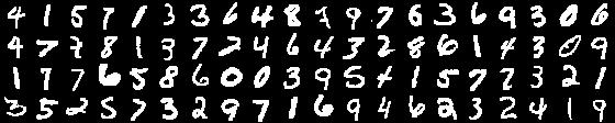
Fig. 1. Examples of images of numbers in the MNIST database
There are many software tools for solving deep learning tasks. In [ 1 ], you can find a general comparison of the functionality of the most famous, here we give general information about some of them ( table 1 ). The first six software libraries implement the widest range of deep learning methods. The developers provide opportunities for creating fully connected neural networks (fully connected neural network, FC NN [ 2 ]), convolutional neural networks (CNN) [ 3 ], auto-encoders (autoencoder, AE) and restricted Boltzmann machines (restricted Boltzmann machine, RBM) [ 4]. It is necessary to pay attention to the remaining libraries. Although they have less functionality, in some cases their simplicity helps to achieve greater performance.
Table 1. Deep Learning Capabilities [ 1 ]
Based on the information given in [ 1 ] and the recommendations of specialists, four libraries were selected for further consideration: Theano , Pylearn2 - one of the most mature and functionally complete libraries, Torch and Caffe - widely used by the community. Each library is considered according to the following plan:
After reviewing the listed libraries, they are compared on a number of test network configurations.
Caffe has been under development since September 2013. The development began with Yangqing Jia during his studies at the University of California at Berkeley. Since then, Caffe has been actively supported by The Berkeley Vision and Learning Center ( BVLC ) and the developer community on GitHub . The library is licensed under BSD 2-Clause.
Caffe is implemented using the C ++ programming language, there are wrappers in Python and MATLAB. The officially supported operating systems are Linux and OS X, and there is also an unofficial port on Windows. Caffe uses the BLAS library (ATLAS, Intel MKL, OpenBLAS) for vector and matrix computing. Along with this, external dependencies include glog, gflags, OpenCV, protoBuf, boost, leveldb, nappy, hdf5, lmdb. To speed up computing, Caffe can be run on the GPU using the basic capabilities of CUDA technology or the cuDNN deep learning primitive library .
Caffe developers support the creation, training, and testing capabilities of fully connected and convolutional neural networks. Input data and transformations are described by the concept of a layer . Depending on the storage format, the following types of source data layers can be used:
Transformations can be defined using layers:
Along with this, various activation functions can be used in the formation of transformations.
The last layer of the neural network model should contain an error function. The library has the following functions:
In the process of training models, various optimization methods are used. Caffe developers provide an implementation of a number of methods:
In the Caffe library, the neural network topology, initial data, and training method are set using configuration files in prototxt format. The file contains a description of the input data (training and test) and layers of the neural network. Let's consider the stages of constructing such files using the example of the “logistic regression” network ( Fig. 2 ). Further, we assume that the file is called linear_regression.prototxt, and it is located in the examples / mnist directory.

Fig. 2. The structure of the neural network
Network configuration is ready. Next, you need to determine the parameters of the training procedure in a file of the prototxt format (let's call it solver.prototxt). The training parameters include the path to the network configuration file (net), the frequency of testing during training (test_interval), stochastic gradient descent parameters (base_lr, weight_decay and others), the maximum number of iterations (max_iter), the architecture on which the calculations will be performed (solver_mode), path to save the trained network (snapshot_prefix).
Training is performed using the main library application. In this case, a certain set of keys is transmitted, in particular, the name of the file containing a description of the parameters of the training procedure.
After training, the resulting model can be used to classify images, for example, using Python wrappers:
Thus, through simple actions, you can get the first results of experiments with deep neural network models. More complex and detailed examples can be seen on the developers website .

Pylearn2 is a library developed at the LISA lab at the University of Montreal since February 2011. He has about 100 developers on GitHub . The library is licensed under BSD 3-Clause.
Pylearn2 is implemented in Python, currently supports the Linux operating system, it is also possible to run on any operating system using a virtual machine, as developers provide a customized wrapper for a virtual environment based on Vagrant. Pylearn2 is an add-on to Theano library . Additionally required are PyYAML, PIL. To speed up the calculations, Pylearn2 and Theano use Cuda-convnet , which is implemented in C ++ / CUDA, which gives a significant increase in speed.
Pylearn2 supports the creation of fully connected and convolutional neural networks, various types of auto-encoders (Contractive Auto-Encoders, Denoising Auto-Encoders) and limited Boltzmann machines (Gaussian RBM, the spike-and-slab RBM). Several error functions are provided: cross-entropy (cross-entropy), log-likelihood (log-likelihood). The following teaching methods are available:
In the Pylearn2 library, neural networks are defined using their description in the configuration file in YAML format. YAML files are a convenient and fast way to serialize objects, as it is developed using object-oriented programming methods.
Consider the procedure for generating YAML files that describe the structure of a neural network and the way it is trained, using the example of logistic regression.
Thus, the network configuration is prepared and the necessary infrastructure for training and classification is determined, which are performed by calling the appropriate Python script. For training, you must run the following command line:
More complex and detailed examples can be seen on the official website or in the repository .

Torch is a library for scientific computing with broad support for machine learning algorithms. Developed by Idiap Research Institute , New York University and NEC Laboratories America , since 2000, distributed under the BSD license.
The library is implemented in Lua using C and CUDA. Fast scripting language Lua in combination with SSE, OpenMP, CUDA technologies allow Torch to show good speed compared to other libraries. Currently supported operating systems are Linux, FreeBSD, Mac OS X. The main modules also work on Windows. Torch dependencies include imagemagick, gnuplot, nodejs, npm, and more.
The library consists of a set of modules, each of which is responsible for various stages of working with neural networks. So, for example, the nn module provides configuration of the neural network (definition of layers and their parameters), the optim module contains implementations of various optimization methods used for training, and gnuplot provides the ability to visualize data (graphing, displaying images, etc.). Installing additional modules allows you to expand the functionality of the library.
Torch allows you to create complex neural networks using the container mechanism. Container- This is a class that combines the declared components of the neural network in one common configuration, which can be transferred to the training procedure in the future. A component of a neural network can be not only fully connected or convolutional layers, but also activation functions or errors, as well as ready-made containers. Torch allows you to create the following layers:
Error Functions: RMS Error (MSE), Cross Entropy (CrossEntropy), etc.
During training, the following optimization methods can be used:
Consider the process of configuring a neural network in Torch. You must first declare a container, then add layers to it. The order of adding layers is important because the output of the (n-1) -th layer will be the input of the nth.
Use and training of a neural network:
Now let's put it all together. In order to train a neural network in the Torch library, you need to write your own training cycle. In it, declare a special function (closure) that will calculate the network response, determine the error value and recalculate the gradients, and pass this closure to the gradient descent function to update the network weights.
where optimState is the gradient descent parameters (learningRate, momentum, weightDecay, etc.). The full training cycle can be seen here .
It is easy to see that the declaration procedure, like the training procedure, takes less than 10 lines of code, which indicates the ease of use of the library. Moreover, the library allows you to work with neural networks at a fairly low level.
Saving and loading a trained network is carried out using special functions:
After downloading, the network can be used for classification or additional training. If you need to know which class the sample element belongs to, then just go through the network and calculate the output:
More complex examples can be found in the training materials for the library .

Theano is an extension of the Python language that allows you to efficiently calculate mathematical expressions containing multidimensional arrays. The library got its name in honor of the name of the wife of the ancient Greek philosopher and mathematician Pythagoras - Feano (or Teano). Theano was developed in the LISA lab to support the rapid development of machine learning algorithms.
The library is implemented in Python, supported on the operating systems Windows, Linux and Mac OS. Theano includes a compiler that translates mathematical expressions written in Python into efficient C or CUDA code.
Theano provides a basic set of tools for configuring and training neural networks. The implementation of multi-layer fully connected networks (Multi-Layer Perceptron), convolutional neural networks (CNN), recurrent neural networks (Recurrent Neural Networks, RNN), auto-encoders and limited Boltzmann machines is possible. Various activation functions are also provided, in particular, sigmoidal, softmax-function, cross-entropy. In the course of training, batch gradient descent (Batch SGD) is used.
Consider the configuration of the neural network in Theano. For convenience, we implement the LogisticRegression class ( Fig. 3), which will contain the variables - the trained parameters W, b and the functions for working with them - counting the network response (y = softmax (Wx + b)) and the error function. Then, to train the neural network, we create the train_model function. For it, it is necessary to describe the methods that determine the error function, the rule for calculating gradients, the method of changing the weights of the neural network, the size and location of the mini-batch sample (the images themselves and the answers for them). After determining all the parameters, the function is compiled and transferred to the training cycle.
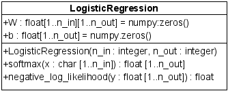
Fig. 3. Class diagram for the implementation of the neural network in Theano
To quickly save and load the parameters of the neural network, you can use the functions from the cPickle package:
It is easy to see that the process of creating a model and determining its parameters requires writing voluminous and noisy code. The library is low level. It is impossible not to note its flexibility, as well as the availability of the possibility of implementing and using its own components. On the official website of the library there is a large number of training materials on various topics.
The following test infrastructure was used in the experiments to evaluate the performance of libraries:
Computational experiments were carried out on fully connected and convolutional neural networks of the following structure:
All weights were initialized randomly according to the uniform distribution law in the range (−6 / (n_in + n_out), 6 / (n_in + n_out)), where n_in, n_out are the number of neurons at the input and output of the layer, respectively. The parameters of stochastic gradient descent (SGD) were chosen equal to the following values: learning rate - 0.01, momentum - 0.9, weight decay - 5e-4, batch size - 128, maximum number of iterations - 150.
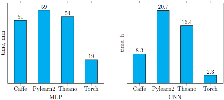
The training time for neural networks described earlier ( Fig. 4 , 5 ) using the four libraries examined is presented below ( Fig. 6 ). It is easy to see that Pylearn2 shows worse performance (both on the CPU and on the GPU) compared to other libraries. As for the rest, the training time is highly dependent on the network structure. The best result among implementations of networks running on the CPU was shown by the Torch library (moreover, on CNN it overtook itself running on the GPU). Among GPU implementations, the best result (on both networks) was shown by the Caffe library. In general, the use of Caffe left only positive impressions.
CPU implementation (see infrastructure ):
GPU implementation (see infrastructure ):
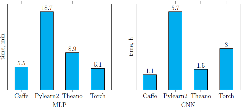
Fig. 6. Training time for MLP and CNN networks described in the previous paragraph.
As for the time for classifying a single image on a CPU using trained models ( Fig. 7 ), it is easy to see that the Torch library was out of competition on both test neural networks. Caffe was a little behind her on CNN, which at the same time showed the worst classification time for MLP.
CPU implementation (see infrastructure ):
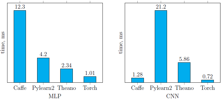
Fig. 7. Classification time for one image using trained MLP and CNN networks.
If we look at the classification accuracy, then on the MLP network it is higher than 97.4%, and CNN - ~ 99% for all libraries ( table 2 ). The obtained accuracy values are somewhat lower than those given on the MNIST website on the same neural network structures. Small differences are due to differences in the settings of the initial weights of the networks and the parameters of the optimization methods used in the learning process. Actually, there was no goal of achieving maximum accuracy values; rather, it was necessary to build identical network structures and set the most similar training parameters.
Table 2. The average value and variance of the classification accuracy indicators for 5 experiments
Based on the study of the library functionality, as well as performance analysis on the example of the task of classifying handwritten numbers, each of them is rated on a scale of 1 to 3 according to the following criteria:
Consider the estimates obtained for each criterion, arrange the places of each library from the first to the third ( table 3 ). According to the results of computational experiments, in terms of speed, the Caffe library is most preferable ( Fig. 6 ). At the same time, it turned out to be the most convenient to use. In terms of flexibility, the Theano library performed best. In terms of functionality, Pylearn2 is the most complete, but its use is complicated by the need to understand the internal device (the formation of YAML files requires this). The most detailed and understandable material for study is provided by the Torch developers. Having shown the average indicators for each criterion separately, it was she who won the ranking of the examined libraries.
Table 3. Library comparison results (places from 1 to 3 for each criterion)
To summarize, we can say that the most mature is the Torch library. At the same time, the Caffe and Theano libraries are not inferior to it in many criteria ( Table 3 ), so the possibility of their subsequent use cannot be ruled out. In the future, it is planned to use the Caffe and Torch libraries to study the applicability of deep learning methods to the tasks of detecting people, pedestrians and cars.
The work was performed in the laboratory "Information Technologies" of the faculty of the VMK NNGU im. N.I. Lobachevsky with the support of Itseez.
Introduction
Currently, machine learning is an actively developing field of scientific research. This is due both to the possibility of faster,
Deep learningconsiders methods for modeling high-level abstractions in data using a variety of sequential nonlinear transformations, which, as a rule, are represented as artificial neural networks. Today, neural networks are successfully used to solve such problems as forecasting, pattern recognition, data compression, and a number of others.
The relevance of the topic of machine learning and, in particular, deep learning is confirmed by the regular appearance of articles on the subject in the Habré:
- Deep learning and Caffe on New Year's holidays.
- Data mining: Toolkit - Theano.
- About cats, dogs, machine learning and deep learning.
- Weekly reviews of the most interesting materials on data analysis and machine learning.
This article is devoted to a comparative analysis of some deep learning software tools, of which a great many have recently appeared [ 1 ]. Among these tools are software libraries, extensions to programming languages, as well as independent languages that allow using ready-made algorithms for creating and training neural network models. Existing deep learning tools have different functionalities and require different levels of knowledge and skills from the user. Choosing the right tool is an important task that allows you to achieve the desired result in the least time and with less effort.
The article provides a brief overview of the tools for designing and training neural network models. Focused on four libraries: Caffe, Pylearn2 , Torch, and Theano . The basic capabilities of these libraries are considered, examples of their use are given. The quality and speed of libraries when comparing the same topologies of neural networks to solve the problem of classifying handwritten numbers is compared (the MNIST dataset is used as a training and test sample ). An attempt is also being made to evaluate the usability of the libraries in question in practice.
MNIST Dataset
Further, the base of the images of handwritten digits MNIST will be used as the studied data set ( Fig. 1 ). Images in this database have a resolution of 28x28 and are stored in grayscale format. The numbers are centered on the image. The entire database is divided into two parts: training, consisting of 50,000 images, and test - 10,000 images.
Fig. 1. Examples of images of numbers in the MNIST database
Software for deep learning tasks
There are many software tools for solving deep learning tasks. In [ 1 ], you can find a general comparison of the functionality of the most famous, here we give general information about some of them ( table 1 ). The first six software libraries implement the widest range of deep learning methods. The developers provide opportunities for creating fully connected neural networks (fully connected neural network, FC NN [ 2 ]), convolutional neural networks (CNN) [ 3 ], auto-encoders (autoencoder, AE) and restricted Boltzmann machines (restricted Boltzmann machine, RBM) [ 4]. It is necessary to pay attention to the remaining libraries. Although they have less functionality, in some cases their simplicity helps to achieve greater performance.
Table 1. Deep Learning Capabilities [ 1 ]
| # | Title | Tongue | OC | FC NN | CNN | Ae | RBM |
| 1 | DeepLearnToolbox | Matlab | Windows Linux | + | + | + | + |
| 2 | Theano | Python | Windows, Linux, Mac | + | + | + | + |
| 3 | Pylearn2 | Python | Linux, Vagrant | + | + | + | + |
| 4 | Deepnet | Python | Linux | + | + | + | + |
| 5 | Deepmat | Matlab | ? | + | + | + | + |
| 6 | Torch | Lua c | Linux, Mac OS X, iOS, Android | + | + | + | + |
| 7 | Darch | R | Windows Linux | + | - | + | + |
| 8 | Caff e | C ++, Python, Matlab | Linux OS X | + | + | - | - |
| 9 | nnForge | C ++ | Linux | + | + | - | - |
| 10 | Cxxnet | C ++ | Linux | + | + | - | - |
| eleven | Cuda-convnet | C ++ | Linux, Windows | + | + | - | - |
| 12 | Cuda CNN | Matlab | Linux, Windows | + | + | - | - |
Based on the information given in [ 1 ] and the recommendations of specialists, four libraries were selected for further consideration: Theano , Pylearn2 - one of the most mature and functionally complete libraries, Torch and Caffe - widely used by the community. Each library is considered according to the following plan:
- Short reference information.
- Technical features (OS, programming language, dependencies).
- Functionality
- An example of the formation of a network such as logistic regression.
- Training and use of the constructed model for classification.
After reviewing the listed libraries, they are compared on a number of test network configurations.
Caffe Library

Caffe has been under development since September 2013. The development began with Yangqing Jia during his studies at the University of California at Berkeley. Since then, Caffe has been actively supported by The Berkeley Vision and Learning Center ( BVLC ) and the developer community on GitHub . The library is licensed under BSD 2-Clause.
Caffe is implemented using the C ++ programming language, there are wrappers in Python and MATLAB. The officially supported operating systems are Linux and OS X, and there is also an unofficial port on Windows. Caffe uses the BLAS library (ATLAS, Intel MKL, OpenBLAS) for vector and matrix computing. Along with this, external dependencies include glog, gflags, OpenCV, protoBuf, boost, leveldb, nappy, hdf5, lmdb. To speed up computing, Caffe can be run on the GPU using the basic capabilities of CUDA technology or the cuDNN deep learning primitive library .
Caffe developers support the creation, training, and testing capabilities of fully connected and convolutional neural networks. Input data and transformations are described by the concept of a layer . Depending on the storage format, the following types of source data layers can be used:
- DATA - defines a data layer in leveldb and lmdb formats.
- HDF5_DATA - data layer in hdf5 format.
- IMAGE_DATA is a simple format that assumes that the file contains a list of images with class labels.
- other.
Transformations can be defined using layers:
- INNER_PRODUCT is a fully connected layer.
- CONVOLUTION - convolutional layer.
- POOLING - a spatial union layer.
- Local Response Normalization (LRN) - a layer of local normalization.
Along with this, various activation functions can be used in the formation of transformations.
- Positive part (Rectified-Linear Unit, ReLU).
- Sigmoid function (SIGMOID).
- Hyperbolic tangent (TANH).
- Absolute value (ABSVAL).
- Extinction (POWER).
- The binomial normal log likelihood function (BNLL).
The last layer of the neural network model should contain an error function. The library has the following functions:
- Mean-square error (MSE).
- Edge error (Hinge loss).
- Logistic loss function.
- Information gain loss function.
- Sigmoid cross entropy loss (Sigmoid cross entropy loss).
- Softmax function. Generalizes sigmoidal cross-entropy to the case of the number of classes more than two.
In the process of training models, various optimization methods are used. Caffe developers provide an implementation of a number of methods:
- Stochastic Gradient Descent (SGD) [ 6 ].
- An adaptive gradient learning rate algorithm (AdaGrad) [ 7 ].
- Nesterov’s Accelerated Gradient Descent (NAG) [ 8 ].
In the Caffe library, the neural network topology, initial data, and training method are set using configuration files in prototxt format. The file contains a description of the input data (training and test) and layers of the neural network. Let's consider the stages of constructing such files using the example of the “logistic regression” network ( Fig. 2 ). Further, we assume that the file is called linear_regression.prototxt, and it is located in the examples / mnist directory.
Fig. 2. The structure of the neural network
- Set the network name.
name: "LinearRegression" - As the training set, the MNIST database is used, stored in lmdb format. To work with lmdb or leveldb formats, a “DATA” type layer is used, in which you need to specify some parameters that describe the input data (data_param): the path to the data on the hard disk (source), data type (backend), and sample size (batch_size). You can also perform various transformations (transform_param) with the data. For example, you can normalize the image by multiplying all values by 0.00390625 (the number inverse to 255). The top parameter specifies one or more names that will be used to identify the output of the layer. In this example, these are processed images (data) and class labels to which the images belong (label).
layers { name: "mnist" type: DATA top: "data" top: "label" data_param { source: "examples/mnist/mnist_train_lmdb" backend: LMDB batch_size: 64 } transform_param { scale: 0.00390625 } } - We define a fully connected layer (the output of each neuron of the previous layer is associated with the input of each neuron of the subsequent layer). A fully connected layer in the Caffe library is defined using a layer of type INNER_PRODUCT. The input name is specified using the bottom parameter. In this layer, the input data are processed images (data). The number of neurons in a layer is determined automatically (by the number of outputs in the previous layer), and the number of output neurons is indicated using the num_output parameter. We put the result of the layer by the same name as the name of the layer (ip).
layers { name: "ip" type: INNER_PRODUCT bottom: "data" top: "ip" inner_product_param { num_output: 10 } } - At the end, add a layer that computes the error function. It takes as input the result of the previous fully connected layer (ip) and class numbers for each image (label). After calculations, the results of this layer can be accessed by the name loss.
layers {
  name: "loss"
  type: SOFTMAX_LOSS
  bottom: "ip"
  bottom: "label"
  top: "loss"
}
Network configuration is ready. Next, you need to determine the parameters of the training procedure in a file of the prototxt format (let's call it solver.prototxt). The training parameters include the path to the network configuration file (net), the frequency of testing during training (test_interval), stochastic gradient descent parameters (base_lr, weight_decay and others), the maximum number of iterations (max_iter), the architecture on which the calculations will be performed (solver_mode), path to save the trained network (snapshot_prefix).
net: "examples/mnist/linear_regression.prototxt"
test_iter: 100
test_interval: 500
base_lr: 0.01
momentum: 0.9
weight_decay: 0.0005
lr_policy: "inv"
gamma: 0.0001
power: 0.75
display: 100
max_iter: 10000
snapshot: 5000
snapshot_prefix: "examples/mnist/linear_regression"
solver_mode: GPU
Training is performed using the main library application. In this case, a certain set of keys is transmitted, in particular, the name of the file containing a description of the parameters of the training procedure.
caffe train --solver=solver.prototxt
After training, the resulting model can be used to classify images, for example, using Python wrappers:
- We connect the Caffe library. Set the test mode and indicate the architecture for performing the calculations (CPU or GPU).
import caffe caffe.set_phase_test() caffe.set_mode_cpu() - We create a neural network, specifying the following parameters: MODEL_FILE - network configuration in prototxt format, PRETRAINED - trained network in caffemodel format, IMAGE_MEAN - average image (calculated from a set of input images and used for subsequent normalization of intensity), channel_swap sets the color model, raw_scale - maximum intensity value, image_dims - image resolution. After that, we load the image for classification (IMAGE_FILE).
net = caffe.Classifier(MODEL_FILE, PRETRAINED, IMAGE_MEAN, channel_swap=(0,1,2), raw_scale=255, image_dims=(28, 28)) input_image = caffe.io.load_image(IMAGE_FILE) - We get the response of the neural network for the selected image and display the results on the screen.
prediction = net.predict([input_image])
print 'prediction shape:', prediction[0].shape
print 'predicted class:', prediction[0].argmax()
Thus, through simple actions, you can get the first results of experiments with deep neural network models. More complex and detailed examples can be seen on the developers website .
Pylearn2 Library
Pylearn2 is a library developed at the LISA lab at the University of Montreal since February 2011. He has about 100 developers on GitHub . The library is licensed under BSD 3-Clause.
Pylearn2 is implemented in Python, currently supports the Linux operating system, it is also possible to run on any operating system using a virtual machine, as developers provide a customized wrapper for a virtual environment based on Vagrant. Pylearn2 is an add-on to Theano library . Additionally required are PyYAML, PIL. To speed up the calculations, Pylearn2 and Theano use Cuda-convnet , which is implemented in C ++ / CUDA, which gives a significant increase in speed.
Pylearn2 supports the creation of fully connected and convolutional neural networks, various types of auto-encoders (Contractive Auto-Encoders, Denoising Auto-Encoders) and limited Boltzmann machines (Gaussian RBM, the spike-and-slab RBM). Several error functions are provided: cross-entropy (cross-entropy), log-likelihood (log-likelihood). The following teaching methods are available:
- Batch Gradient Descent (BGD).
- Stochastic Gradient Descent (SGD).
- Nonlinear conjugate gradient descent (NCG).
In the Pylearn2 library, neural networks are defined using their description in the configuration file in YAML format. YAML files are a convenient and fast way to serialize objects, as it is developed using object-oriented programming methods.
Consider the procedure for generating YAML files that describe the structure of a neural network and the way it is trained, using the example of logistic regression.
- Define a training set. Pylearn2 already has a class for working with the MNIST database. We will train on the first 50,000 images.
!obj:pylearn2.train.Train { dataset: &train !obj:pylearn2.datasets.mnist.MNIST { which_set: 'train', one_hot: 1, start: 0, stop: 50000 }, - We describe the network structure. For this we use a class that implements logistic regression. It is enough to specify the necessary parameters. The number of input neurons in a fully connected layer (nvis) is 784 (by the number of pixels in the image), output (n_classes) - 10 (by the number of classes of objects), initial weights (iranges) are determined by zeros.
model: !obj:pylearn2.models.softmax_regression.SoftmaxRegression { n_classes: 10, irange: 0., nvis: 784, }, - We choose the neural network learning algorithm and its parameters. For training, we choose the method of batch gradient descent (BGD). The batch_size parameter is responsible for the size of the training sample used at each step of the gradient descent. Setting line_search_mode to exhaustive means the batch gradient descent (BGD) method will try to use binary search to reach the best point along the gradient direction, which speeds up the convergence of the gradient descent. During the training, we will track the classification results in the training, validation (images from 50,000 to 60,000) and test samples. Stop criterion - maximum number of optimization iterations.
algorithm: !obj:pylearn2.training_algorithms.bgd.BGD { batch_size: 128, line_search_mode: 'exhaustive', monitoring_dataset: { 'train' : *train, 'valid' : !obj:pylearn2.datasets.mnist.MNIST { which_set: 'train', one_hot: 1, start: 50000, stop: 60000 }, 'test' : !obj:pylearn2.datasets.mnist.MNIST { which_set: 'test', one_hot: 1, } }, termination_criterion: !obj:pylearn2.termination_criteria.And { criteria: [ !obj:pylearn2.termination_criteria.EpochCounter { max_epochs: 150 }, ] } }, - For further use of the trained model, it is necessary to save the result. Note that the model is saved in pkl format.
extensions: [
    !obj:pylearn2.train_extensions.best_params.MonitorBasedSaveBest {
    channel_name: 'valid_y_misclass',
    save_path: "%(save_path)s/softmax_regression_best.pkl"
  },
]
Thus, the network configuration is prepared and the necessary infrastructure for training and classification is determined, which are performed by calling the appropriate Python script. For training, you must run the following command line:
python train.py <файл с конфигурацией сети>.yamlMore complex and detailed examples can be seen on the official website or in the repository .
Library torch
Torch is a library for scientific computing with broad support for machine learning algorithms. Developed by Idiap Research Institute , New York University and NEC Laboratories America , since 2000, distributed under the BSD license.
The library is implemented in Lua using C and CUDA. Fast scripting language Lua in combination with SSE, OpenMP, CUDA technologies allow Torch to show good speed compared to other libraries. Currently supported operating systems are Linux, FreeBSD, Mac OS X. The main modules also work on Windows. Torch dependencies include imagemagick, gnuplot, nodejs, npm, and more.
The library consists of a set of modules, each of which is responsible for various stages of working with neural networks. So, for example, the nn module provides configuration of the neural network (definition of layers and their parameters), the optim module contains implementations of various optimization methods used for training, and gnuplot provides the ability to visualize data (graphing, displaying images, etc.). Installing additional modules allows you to expand the functionality of the library.
Torch allows you to create complex neural networks using the container mechanism. Container- This is a class that combines the declared components of the neural network in one common configuration, which can be transferred to the training procedure in the future. A component of a neural network can be not only fully connected or convolutional layers, but also activation functions or errors, as well as ready-made containers. Torch allows you to create the following layers:
- Fully connected layer (Linear).
- Activation functions: hyperbolic tangent (Tanh), selection of minimum (Min) or maximum (Max), softmax-function (SoftMax) and others.
- Convolutional layers: convolution (Convolution), thinning (SubSampling), spatial union (MaxPooling, AveragePooling, LPPooling), difference normalization (SubtractiveNormalization).
Error Functions: RMS Error (MSE), Cross Entropy (CrossEntropy), etc.
During training, the following optimization methods can be used:
- Stochastic Gradient Descent (SGD),
- Averaged stochastic gradient descent (Averaged SGD) [ 9 ].
- The Bruden – Fletcher – Goldfarb – Channo (L-BFGS) algorithm [ 10 ].
- Conjugate Gradient (CG).
Consider the process of configuring a neural network in Torch. You must first declare a container, then add layers to it. The order of adding layers is important because the output of the (n-1) -th layer will be the input of the nth.
regression = nn.Sequential()
regression:add(nn.Linear(784,10))
regression:add(nn.SoftMax())
loss = nn.ClassNLLCriterion()
Use and training of a neural network:
- Загрузка входных данных X. Функция torch.load(path_to_ready_dset) позволяет загрузить подготовленный заранее датасет в текстовом или бинарном формате. Как правило, это Lua-таблица состоящая из трёх полей: размер, данные и метки. В случае если готового датасета нет, можно воспользоваться стандартными функциями языка Lua (например, io.open(filename [, mode])) или функциями из пакетов библиотеки Torch (например, image.loadJPG(filename)).
- Определение ответа сети для входных данных X:
Y = regression:forward(X) - Вычисление функции ошибки E = loss(Y,T), в нашем случае это функция правдоподобия.
E = loss:forward(Y,T) - Просчет градиентов согласно алгоритму обратного распространения.
dE_dY = loss:backward(Y,T)
regression:backward(X,dE_dY)
Now let's put it all together. In order to train a neural network in the Torch library, you need to write your own training cycle. In it, declare a special function (closure) that will calculate the network response, determine the error value and recalculate the gradients, and pass this closure to the gradient descent function to update the network weights.
-- Создаём специальные переменные: веса нейросети и их градиенты
w, dE_dw = regression:getParameters()
local eval_E = function(w)
    dE_dw:zero() -- Обновляем градиенты
    local Y = regression:forward(X)
    local E = loss:forward(Y,T)
    local dE_dY = loss:backward(Y,T)
    regression:backward(X,dE_dY)
    return E, dE_dw
end
-- Затем в цикле обучения вызываем
optim.sgd(eval_E, w, optimState)
where optimState is the gradient descent parameters (learningRate, momentum, weightDecay, etc.). The full training cycle can be seen here .
It is easy to see that the declaration procedure, like the training procedure, takes less than 10 lines of code, which indicates the ease of use of the library. Moreover, the library allows you to work with neural networks at a fairly low level.
Saving and loading a trained network is carried out using special functions:
torch.save(path, regression)
net = torch.load(path)
After downloading, the network can be used for classification or additional training. If you need to know which class the sample element belongs to, then just go through the network and calculate the output:
result = net:forward(sample)
More complex examples can be found in the training materials for the library .
Theano Library
Theano is an extension of the Python language that allows you to efficiently calculate mathematical expressions containing multidimensional arrays. The library got its name in honor of the name of the wife of the ancient Greek philosopher and mathematician Pythagoras - Feano (or Teano). Theano was developed in the LISA lab to support the rapid development of machine learning algorithms.
The library is implemented in Python, supported on the operating systems Windows, Linux and Mac OS. Theano includes a compiler that translates mathematical expressions written in Python into efficient C or CUDA code.
Theano provides a basic set of tools for configuring and training neural networks. The implementation of multi-layer fully connected networks (Multi-Layer Perceptron), convolutional neural networks (CNN), recurrent neural networks (Recurrent Neural Networks, RNN), auto-encoders and limited Boltzmann machines is possible. Various activation functions are also provided, in particular, sigmoidal, softmax-function, cross-entropy. In the course of training, batch gradient descent (Batch SGD) is used.
Consider the configuration of the neural network in Theano. For convenience, we implement the LogisticRegression class ( Fig. 3), which will contain the variables - the trained parameters W, b and the functions for working with them - counting the network response (y = softmax (Wx + b)) and the error function. Then, to train the neural network, we create the train_model function. For it, it is necessary to describe the methods that determine the error function, the rule for calculating gradients, the method of changing the weights of the neural network, the size and location of the mini-batch sample (the images themselves and the answers for them). After determining all the parameters, the function is compiled and transferred to the training cycle.
Fig. 3. Class diagram for the implementation of the neural network in Theano
Software implementation of the class
class LogisticRegression(object):
    def __init__(self, input, n_in, n_out):
 # y = W * x + b
 # объявляем переменные, определяем тип, количество входов и выходов
        self.W = theano.shared(
       # инициализируем начальные веса нулями
        	value=numpy.zeros((n_in, n_out), dtype=theano.config.floatX), name='W', borrow=True)
        self.b = theano.shared(value=numpy.zeros((n_out,), dtype=theano.config.floatX), name='b', borrow=True)
 # добавляем функцию активации softmax, выход сети - переменная y_pred
        self.p_y_given_x = T.nnet.softmax(T.dot(input, self.W) + self.b)
        self.y_pred = T.argmax(self.p_y_given_x, axis=1)
        self.params = [self.W, self.b]
    # определяем функцию ошибки
    def negative_log_likelihood(self, y):
        return -T.mean(T.log(self.p_y_given_x)[T.arange(y.shape[0]), y])
# x - подается на вход сети
# набор изображений (minibatch) располагается по строкам в матрице x
# y - ответ сети на каждый семпл
x = T.matrix('x')
y = T.ivector('y')
# создаем модель логистической регрессии каждое MNIST изображение имеет размер 28*28
classifier = LogisticRegression(input=x, n_in=28 * 28, n_out=10)
# значение функции ошибки, которое мы пытаемся минимизировать в течение обучения
cost = classifier.negative_log_likelihood(y)
# чтобы посчитать градиенты, необходимо вызвать функцию Theano - grad
g_W = T.grad(cost=cost, wrt=classifier.W)
g_b = T.grad(cost=cost, wrt=classifier.b)
# определяем правила обновления весов нейросети
updates = [(classifier.W, classifier.W - learning_rate * g_W),  (classifier.b, classifier.b - learning_rate * g_b)]
# компилируем функцию тренировки, в дальнейшем она будет вызываться в цикле обучения
train_model = theano.function(
    inputs=[index], outputs=cost, updates=updates,
    givens={
        x: train_set_x[index * batch_size: (index + 1) * batch_size],
        y: train_set_y[index * batch_size: (index + 1) * batch_size]
    }
)
To quickly save and load the parameters of the neural network, you can use the functions from the cPickle package:
import cPickle
save_file = open('path', 'wb')
cPickle.dump(classifier.W.get_value(borrow=True), save_file, -1)
cPickle.dump(classifier.b.get_value(borrow=True), save_file, -1)
save_file.close()
file = open('path')
classifier.W.set_value(cPickle.load(save_file), borrow=True)
classifier.b.set_value(cPickle.load(save_file), borrow=True)
It is easy to see that the process of creating a model and determining its parameters requires writing voluminous and noisy code. The library is low level. It is impossible not to note its flexibility, as well as the availability of the possibility of implementing and using its own components. On the official website of the library there is a large number of training materials on various topics.
Comparison of libraries on the example of the task of classifying handwritten numbers
Test infrastructure
The following test infrastructure was used in the experiments to evaluate the performance of libraries:
- Ubuntu 12.04, Intel Core i5-3210M @ 2.5GHz (CPU experiments).
- Ubuntu 14.04, Intel Core i5-2430M @ 2.4GHz + NVIDIA GeForce GT 540M (GPU experiments).
- GCC 4.8, NVCC 6.5.
Network Topologies and Learning Options
Computational experiments were carried out on fully connected and convolutional neural networks of the following structure:
- Three-layer fully connected neural network (MLP, Fig. 4 ):
- 1st layer - FC (in: 784, out: 392, activation: tanh).
- 2d layer - FC (in: 392, out: 196, activation: tanh).
- 3d layer - FC (in: 196, out: 10, activation: softmax).
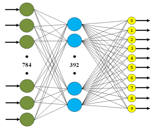
Fig. 4. The structure of a three-layer fully connected network - Convolutional neural network (CNN, Fig. 5 ):
- 1st layer - convolution (in filters: 1, out filters: 28, size: 5x5, stride: 1x1).
- 2d layer - max-pooling (size: 3x3, stride: 3x3).
- 3d layer - convolution (in filters: 28, out filters: 56, size: 5x5, stride 1x1).
- 4th layer - max-pooling (size: 2x2, stride: 2x2).
- 5th layer - FC (in: 224, out: 200, activation: tanh).
- 6th layer - FC (in: 200, out: 10, activation: softmax).
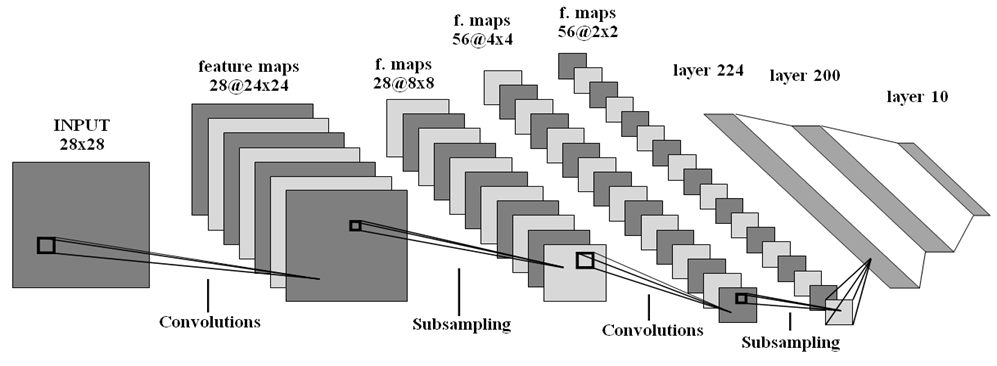
Fig. 5. The structure of the convolutional neural network
All weights were initialized randomly according to the uniform distribution law in the range (−6 / (n_in + n_out), 6 / (n_in + n_out)), where n_in, n_out are the number of neurons at the input and output of the layer, respectively. The parameters of stochastic gradient descent (SGD) were chosen equal to the following values: learning rate - 0.01, momentum - 0.9, weight decay - 5e-4, batch size - 128, maximum number of iterations - 150.
Experiment Results
The training time for neural networks described earlier ( Fig. 4 , 5 ) using the four libraries examined is presented below ( Fig. 6 ). It is easy to see that Pylearn2 shows worse performance (both on the CPU and on the GPU) compared to other libraries. As for the rest, the training time is highly dependent on the network structure. The best result among implementations of networks running on the CPU was shown by the Torch library (moreover, on CNN it overtook itself running on the GPU). Among GPU implementations, the best result (on both networks) was shown by the Caffe library. In general, the use of Caffe left only positive impressions.
CPU implementation (see infrastructure ):
GPU implementation (see infrastructure ):
Fig. 6. Training time for MLP and CNN networks described in the previous paragraph.
As for the time for classifying a single image on a CPU using trained models ( Fig. 7 ), it is easy to see that the Torch library was out of competition on both test neural networks. Caffe was a little behind her on CNN, which at the same time showed the worst classification time for MLP.
CPU implementation (see infrastructure ):
Fig. 7. Classification time for one image using trained MLP and CNN networks.
If we look at the classification accuracy, then on the MLP network it is higher than 97.4%, and CNN - ~ 99% for all libraries ( table 2 ). The obtained accuracy values are somewhat lower than those given on the MNIST website on the same neural network structures. Small differences are due to differences in the settings of the initial weights of the networks and the parameters of the optimization methods used in the learning process. Actually, there was no goal of achieving maximum accuracy values; rather, it was necessary to build identical network structures and set the most similar training parameters.
Table 2. The average value and variance of the classification accuracy indicators for 5 experiments
| Caffe | Pylearn2 | Theano | Torch | |||||
| Accuracy % | Dispersion | Accuracy % | Dispersion | Accuracy % | Dispersion | Accuracy % | Dispersion | |
| MLP | 98.26 | 0.0039 | 98.1 | 0 | 97.42 | 0.0023 | 98.19 | 0 |
| CNN | 99.1 | 0.0038 | 99.3 | 0 | 99.16 | 0.0132 | 99.4 | 0 |
Compare selected libraries
Based on the study of the library functionality, as well as performance analysis on the example of the task of classifying handwritten numbers, each of them is rated on a scale of 1 to 3 according to the following criteria:
- The learning speed reflects the learning time of the neural network models considered at the stage of the experiments.
- The classification speed reflects the classification time of a single image.
- Ease of use is a criterion that allows you to evaluate the time spent studying the library.
- The flexibility of setting up connections between layers, setting method parameters, as well as the availability of various methods of data processing.
- Объем функционала — наличие реализации типовых методов глубокого обучения (полностью связанных сетей, сверточных нейросетей, автокодировщиков, ограниченных машин Больцмана, различных методов оптимизации и функций ошибки).
- Наличие и удобство использования документации и обучающих материалов
Consider the estimates obtained for each criterion, arrange the places of each library from the first to the third ( table 3 ). According to the results of computational experiments, in terms of speed, the Caffe library is most preferable ( Fig. 6 ). At the same time, it turned out to be the most convenient to use. In terms of flexibility, the Theano library performed best. In terms of functionality, Pylearn2 is the most complete, but its use is complicated by the need to understand the internal device (the formation of YAML files requires this). The most detailed and understandable material for study is provided by the Torch developers. Having shown the average indicators for each criterion separately, it was she who won the ranking of the examined libraries.
Table 3. Library comparison results (places from 1 to 3 for each criterion)
| Learning speed | Classification rate | Convenience | Flexibility | Functional | Documentation | Amount | |
| Caffe | 1 | 2 | 1 | 3 | 3 | 2 | 12 |
| Pylearn2 | 3 | 3 | 2 | 3 | 1 | 3 | fifteen |
| Torch | 2 | 1 | 2 | 2 | 2 | 1 | 10 |
| Theano | 2 | 2 | 3 | 1 | 2 | 2 | 12 |
Conclusion
To summarize, we can say that the most mature is the Torch library. At the same time, the Caffe and Theano libraries are not inferior to it in many criteria ( Table 3 ), so the possibility of their subsequent use cannot be ruled out. In the future, it is planned to use the Caffe and Torch libraries to study the applicability of deep learning methods to the tasks of detecting people, pedestrians and cars.
The work was performed in the laboratory "Information Technologies" of the faculty of the VMK NNGU im. N.I. Lobachevsky with the support of Itseez.
Used sources
- Kustikova, V.D., Druzhkov, P.N.: A Survey of Deep Learning Methods and Software for Image Classification and Object Detection. In: Proc. of the 9th Open German-Russian Workshop on Pattern Recognition and Image Understanding. (2014)
- Hinton, G.E.: Learning Multiple Layers of Representation. In: Trends in Cognitive Sciences. Vol. 11. pp. 428-434. (2007)
- LeCun, Y., Kavukcuoglu, K., Farabet, C.: Convolutional networks and applications in vision. In: Proc. of the IEEE Int. Symposium on Circuits and Systems (ISCAS). pp. 253-256. (2010)
- Hayat, M., Bennamoun, M., An, S.: Learning Non-Linear Reconstruction Models for Image Set Classification. In: Proc. of the IEEE Conf. on Computer Vision and Pattern Recognition. (2014)
- Restricted Boltzmann Machines (RBMs), www.deeplearning.net/tutorial/rbm.html.
- Bottou, L.: Stochastic Gradient Descent Tricks. Neural Networks: Tricks of the Trade, research.microsoft.com/pubs/192769/tricks-2012.pdf.
- Duchi, J., Hazan, E., Singer, Y.: Adaptive Subgradient Methods for Online Learning and Stochastic Optimization. In: The Journal of Machine Learning Research. (2011)
- Sutskever, I., Martens, J., Dahl, G., Hinton, G.: On the Importance of Initialization and Momentum in Deep Learning. In: Proc. of the 30th Int. Conf. on Machine Learning. (2013)
- Усредненный стохастический градиентный спуск (ASGD), research.microsoft.com/pubs/192769/tricks-2012.pdf.
- Алгоритм Бройдена-Флетчера-Гольдфарба-Шанно, en.wikipedia.org/wiki/Limited-memory_BFGS.