Kalman Filter as Observer: Formulas and Application

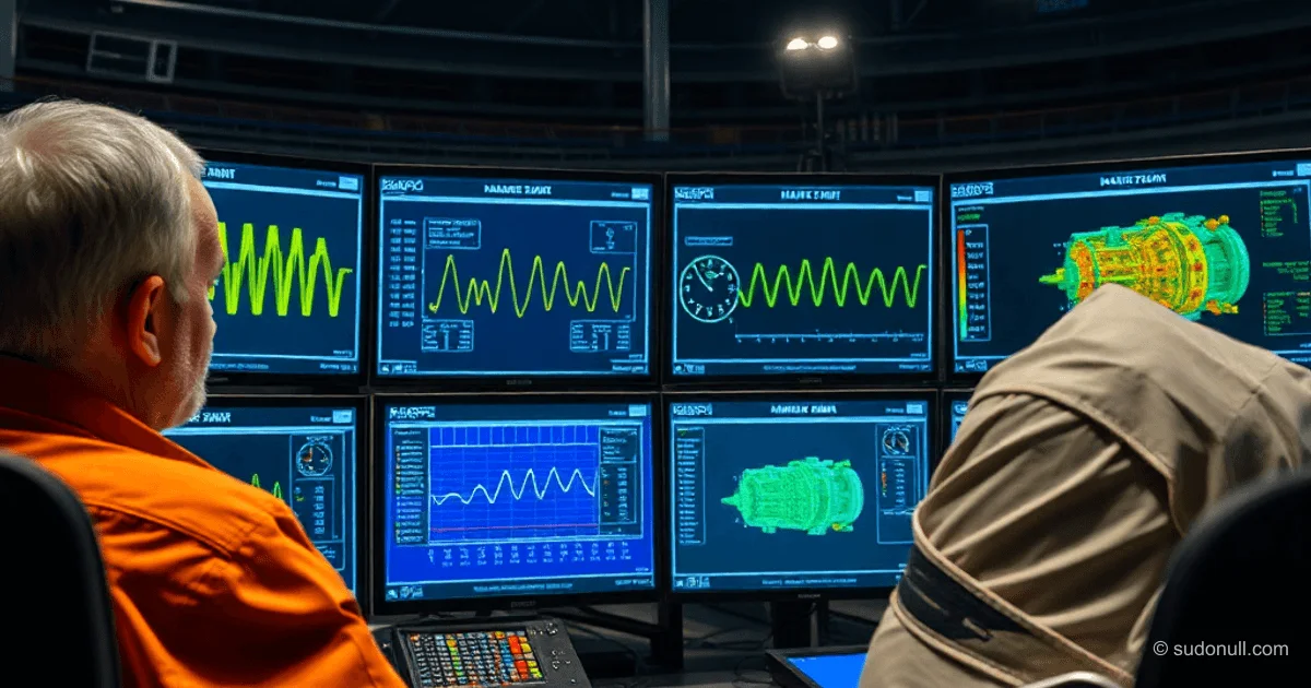
The Observer as a Stochastic Kalman Filter: Mathematical Connection

The Kalman filter implements optimal observation of dynamic systems through stochastic state correction. In the context of modeling a submersible pump's electric motor, phase voltages serve as the model input, while currents act as measurements to synchronize the virtual model with the real object. This enables the extraction of parameters not directly accessible, such as rotor speed.

Mathematical model for state prediction:

\begin{align}
  & \hat{x}_k = F_k \hat{x}_{k-1} + B_k \vec{u}_k \\
  & P_k = F_k P_{k-1} F_k^T + Q_k
\end{align} \tag{1}

Here, $F_k$ is the discrete-time system dynamics matrix (electric motor), $\hat{x}_k$ is the estimated state vector with covariance $P_k = Cov(\hat{x}_k)$, $Q_k$ is the process noise covariance (disturbances from non-uniform oil fractions), $\vec{u}_k$ are deterministic inputs (phase voltages), and $B_k$ is the input matrix.

Correction Based on Measurements

Predicted quasi-sensor currents: $\vec{\mu}_{expected} = H_k \hat{x}_k$, with covariance $\Sigma_{expected} = H_k P_k H_k^T$. Actual current measurements: $\vec{z}_k$ with covariance $R_k = Cov(\vec{z}_k)$.

Combining prediction and measurement via Gaussian product yields corrected estimates:

\begin{align}
  & \vec{\mu}' = \vec{\mu}_0 + K(\vec{\mu}_1 - \vec{\mu}_0) \\
  & \Sigma' = \Sigma_0 - K \Sigma_0 \\
  & K = \Sigma_0 (\Sigma_0 + \Sigma_1)^{-1}
\end{align} \tag{4}

Where $(\vec{\mu}_0, \Sigma_0) = (H_k \hat{x}_k, H_k P_k H_k^T)$, $(\vec{\mu}_1, \Sigma_1) = (\vec{z}_k, R_k)$. Connection to state space:

\begin{align}
  & \vec{\mu}' = H_k \hat{x}'_k \\
  & \Sigma' = H_k P'_k H_k^T
\end{align} \tag{5}

Substitution leads to standard Kalman correction formulas:

\begin{align}
  & \hat{x}'_k = \hat{x}_k + K'_k (\vec{z}_k - H_k \hat{x}_k) \\
  & P'_k = P_k - K'_k H_k P_k \\
  & K'_k = P_k H_k^T (H_k P_k H_k^T + R_k)^{-1}
\end{align} \tag{8}

Canonical Observer Form

Full iteration scheme: prediction via (1), correction via (8), then $\hat{x}_{k-1} \leftarrow \hat{x}'_k$, $P_{k-1} \leftarrow P'_k$. Substituting prediction into correction yields the canonical observer:

\hat{x}'_k = F_k \hat{x}_{k-1} + B_k \vec{u}_k + K'_k (\vec{z}_k - H_k \hat{x}_k)

• $F_k \hat{x}_{k-1} + B_k \vec{u}_k$: object model with inputs (voltages).
• $\vec{z}_k$: measurements (currents).
• $K'_k (\vec{z}_k - H_k \hat{x}_k)$: correction minimizing error $\vec{z}_k - H_k \hat{x}_k \to 0$.

As a result, the model's virtual currents synchronize with real ones, and coordinates $\hat{x}'_k$ reflect true states, including rotor speed.

Key advantages for middle/senior developers:

• Stochastic interpretation: Covariances $P_k$, $Q_k$, $R_k$ account for model and measurement uncertainties.
• Recursiveness: Iterative algorithm suits real-time systems (DSP, embedded).
• Optimality: Minimizes mean squared estimation error under Gaussian noise.
• Scalability: Easily adaptable to nonlinear cases (EKF/UKF).

Key Takeaways

• The Kalman filter is equivalent to an optimal stochastic observer for linear systems with additive noise.
• The correction term $K'_k$ ensures model synchronization with reality by minimizing innovations $\vec{z}_k - H_k \hat{x}_k$.
• Application to electric motors: virtual tachometer based on currents/voltages without a physical speed sensor.
• The observation problem in stochastic settings equals a filtering problem; Kalman is a special case of Bayesian recursion.

— Editorial Team