Making a machine learning project in Python. Part 2
- Transfer
- Tutorial

Translation A Complete Machine Learning Walk-Through in
Python: Part Two piece together all the parts of machine learning project is very difficult. In this series of articles, we will go through all the steps of implementing a machine learning process using real data, and find out how different techniques combine with each other.
In the first article, we cleaned and structured the data, conducted an exploratory analysis, collected a set of attributes for use in the model, and established a baseline for evaluating the results. With this article, we will learn how to implement in Python and compare several machine learning models, conduct hyperparameter tuning to optimize the best model, and evaluate the performance of the final model on a test dataset.
The entire project code is on GitHub , and here is the second notebook related to the current article. You can use and modify the code on your own!
Evaluation and selection of a model
Memo: we are working on a controlled regression problem, we use information on the energy consumption of buildings in New York to create a model that predicts what Energy Star Score a building will receive. We are interested in both the accuracy of prediction and the interpretability of the model.
Today, you can choose from a variety of machine learning models available , and this abundance is intimidating. Of course, there are comparative reviews on the net that will help you navigate when choosing an algorithm, but I prefer to try a few at work and see which one is better. Machine learning for the most part is based on empirical rather than theoretical results , and practicallyit is impossible to understand in advance which model will be more accurate .
It is usually recommended to start with simple, interpretable models, such as linear regression, and if the results are unsatisfactory, then move to more complex, but usually more accurate methods. This graph (very unscientific) shows the relationship between the accuracy and interpretability of some algorithms:

Interpretability and accuracy ( Source ).
We will evaluate five models of varying degrees of complexity:
- Linear regression.
- The method of k-nearest neighbors.
- "Random Forest."
- Gradient boosting.
- Support vector machine.
We will consider not the theoretical apparatus of these models, but their implementation. If you are interested in theory, you can read An Introduction to Statistical Learning (available for free) or Hands-On Machine Learning with Scikit-Learn and TensorFlow . In both books, the theory is beautifully explained and the effectiveness of using the methods mentioned in R and Python, respectively, is shown.
Fill in the missing values
Although during data cleansing we dropped the columns that lack more than half of the values, we still lack many values. Machine learning models cannot work with missing data, so we need to fill it in .
First, we count the data and remember what it looks like:
import pandas as pd
import numpy as np
# Read in data into dataframes
train_features = pd.read_csv('data/training_features.csv')
test_features = pd.read_csv('data/testing_features.csv')
train_labels = pd.read_csv('data/training_labels.csv')
test_labels = pd.read_csv('data/testing_labels.csv')
Training Feature Size:  (6622, 64)
Testing Feature Size:   (2839, 64)
Training Labels Size:   (6622, 1)
Testing Labels Size:    (2839, 1)
Each
NaNvalue is a missing record in the data. You can fill them in different ways , and we will use a fairly simple method of median filling (median imputation), which replaces the missing data with average values for the corresponding columns. In the code below, we will create a Scikit-Learn object
Imputerwith a median strategy. Then we will train it on training data (with help imputer.fit), and apply it to fill in the missing values in the training and test sets (with help imputer.transform). That is, the records that are missing in the test data will be filled with the corresponding median value from the training data .We do the filling and do not train the model on the data as it is, in order to avoid problems with leakage of test data , when information from the test dataset passes into the training one.
# Create an imputer object with a median filling strategy
imputer = Imputer(strategy='median')
# Train on the training features
imputer.fit(train_features)
# Transform both training data and testing data
X = imputer.transform(train_features)
X_test = imputer.transform(test_features)
Missing values in training features:  0
Missing values in testing features:   0
Now all values are filled, no gaps.
Feature scaling
Scaling is the general process of changing the range of a feature. This is a necessary step , because the signs are measured in different units, which means they cover different ranges. This greatly distorts the results of such algorithms as the support vector machine and the k-nearest neighbor method, which take into account the distances between measurements. And scaling allows to avoid it. And although methods like linear regression and the “random forest” do not require scaling of features, it is better not to neglect this step when comparing several algorithms.
We will scale by casting each attribute to the range from 0 to 1. Take all the values of the attribute, select the minimum and divide it by the difference between the maximum and minimum (range). This method of scaling is often called normalization, and the other main method is standardization .
This process is easy to implement manually, so
MinMaxScalerlet's use an object from Scikit-Learn. The code for this method is identical to the code for filling in the missing values, only scaling is used instead of the insert. Recall that we teach the model only on the training set, and then convert all the data.# Create the scaler object with a range of 0-1
scaler = MinMaxScaler(feature_range=(0, 1))
# Fit on the training data
scaler.fit(X)
# Transform both the training and testing data
X = scaler.transform(X)
X_test = scaler.transform(X_test)Now, for every attribute, the minimum value is 0, and the maximum is 1. Filling in the missing values and scaling of the signs — these two steps are needed in almost any machine learning process.
We implement machine learning models in Scikit-Learn
After all the preparatory work, the process of creating, training and running models is relatively simple. We will use the Scikit-Learn library in Python , well-documented and with a well-thought-out syntax for building models. By learning how to create a model in Scikit-Learn, you can quickly implement all sorts of algorithms.
To illustrate the process of creation, learning (
.fit) and testing ( .predict) we will be using gradient boosting:from sklearn.ensemble import GradientBoostingRegressor
# Create the model
gradient_boosted = GradientBoostingRegressor()
# Fit the model on the training data
gradient_boosted.fit(X, y)
# Make predictions on the test data
predictions = gradient_boosted.predict(X_test)
# Evaluate the model
mae = np.mean(abs(predictions - y_test))
print('Gradient Boosted Performance on the test set: MAE = %0.4f' % mae)
Gradient Boosted Performance on the test set: MAE = 10.0132Only one line of code to create, train, and test. To build other models, we use the same syntax, changing only the name of the algorithm.
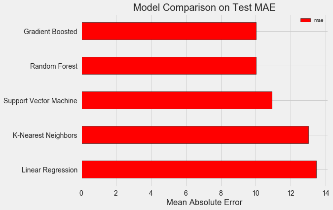
In order to objectively evaluate the models, we calculated the base level using the median value of the target and obtained 24.5. And the results were much better, so that our problem can be solved using machine learning.
In our case, the gradient boosting (MAE = 10,013) turned out to be slightly better than the “random forest” (10,014 MAE). Although these results can not be considered completely honest, because for hyper parameters we mostly use the default values. The effectiveness of the models depends heavily on these settings, especially in the support vector machine.. Nevertheless, based on these results, we will choose a gradient boosting and optimize it.
Hyperparametric model optimization
After choosing a model, you can optimize it for the problem being solved by setting up hyper parameters.
But first of all, let's see what hyperparameters are and how do they differ from ordinary parameters ?
- Hyperparameters of the model can be considered the settings of the algorithm, which we set before the start of its training. For example, the hyperparameter is the number of trees in a “random forest”, or the number of neighbors in the k-nearest neighbors method.
- The model parameters are what she learns during training, for example, weights in linear regression.
By controlling the hyperparameter, we influence the results of the model, changing the balance between its under-training and re-training . Under-training is a situation when a model is not sufficiently complex (it has too few degrees of freedom) to study the correspondence of features and purpose. The under-trained model has a high bias, which can be corrected by complicating the model.
Retraining is the situation when a model essentially memorizes training data. The retrained model has a high variance, which can be corrected by limiting the complexity of the model through regularization. Both under-trained and over-trained models will not be able to generalize well the test data.
The difficulty in choosing the right hyperparameters is that for each task there will be a unique optimal set. Therefore, the only way to choose the best settings is to try different combinations on the new dataset. Fortunately, Scikit-Learn has a number of methods for effectively evaluating hyperparameters. Moreover, in projects like TPOT, attempts are being made to optimize the search for hyperparameters using approaches such as genetic programming . In this article we will limit the use of Scikit-Learn.
Random search with crosscheck
Let's implement the method of setting up hyper parameters, which is called random cross-search searches:
- Random search is a method of choosing hyper parameters. We define a grid, and then randomly select different combinations from it, unlike grid search, in which we sequentially try each combination. By the way, random search works almost as well as the grid , but much faster.
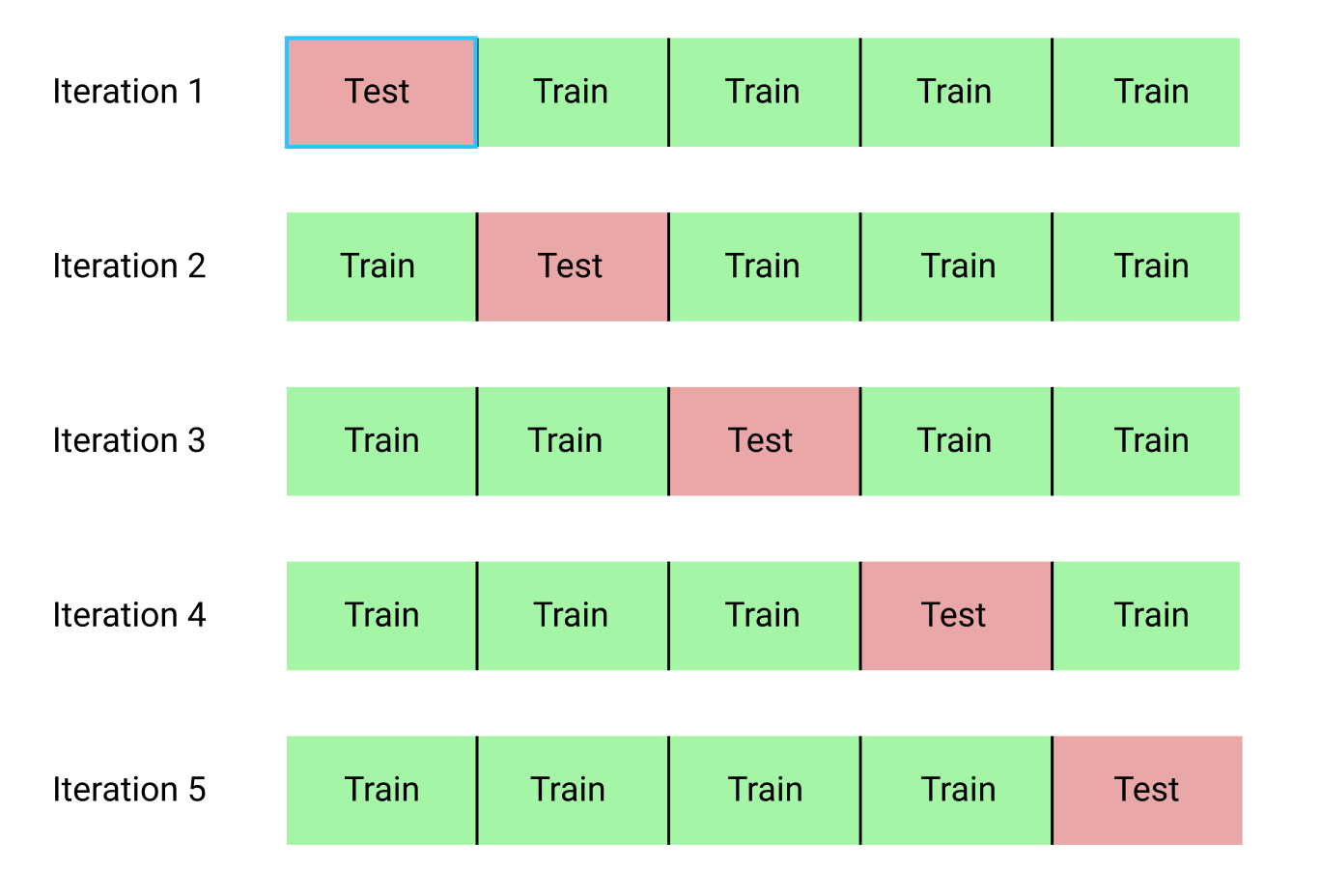
- Cross checking is a method for evaluating a selected combination of hyperparameters. Instead of dividing the data into training and test sets, which reduces the amount of data available for training, we will use the K-Fold Cross Validation. To do this, we divide the training data into k blocks, and then run an iterative process, during which we first train the model on k-1 blocks, and then compare the result when training on the k-th block. We will repeat the process k times, and at the end we will get the average error value for each iteration. This will be the final assessment.
Here is a vivid illustration of the k-block cross-check with k = 5:
The whole process of a random search with cross-check looks like this:
- Set the grid of hyperparameters.
- Randomly select a combination of hyperparameters.
- Create a model using this combination.
- We estimate the result of the model using a k-block cross check.
- We decide which hyperparameters give the best result.
Of course, all this is not done manually, but with the help
RandomizedSearchCVof Scikit-Learn!A small digression: Gradient boosting methods
We will use a regression model based on gradient boosting. This is a composite method, that is, the model consists of numerous "weak learners" (weak learners), in this case from individual decision trees (decision trees). If pupils learn in parallel algorithms like “random forest” , then the prediction result is selected by voting, then in boosting algorithms like gradient boosting, students learn successively, and each of them “focuses” on the mistakes made by the predecessors.
In recent years, boosting algorithms have become popular and often win machine learning contests. Gradient boosting- one of the implementations in which to minimize the cost of the function is applied gradient descent (Gradient Descent). The implementation of gradient boosting in Scikit-Learn is considered not as effective as in other libraries, for example, in XGBoost , but it works well on small datasets and gives fairly accurate predictions.
Back to hyperparameter tuning
There are many hyperparameters in the regression using gradient boosting that need to be customized, refer you to the Scikit-Learn documentation for details. We will optimize:
loss: minimizing loss function;n_estimators: the number of weak decision trees used;max_depth: maximum depth of each decision tree;min_samples_leaf: the minimum number of examples that should be in the "leaf" (leaf) node of the decision tree;min_samples_split: The minimum number of examples that are needed to separate the node in the decision tree;max_features: The maximum number of attributes that are used to separate nodes.
I'm not sure that at least someone really understands how it all works, and the only way to find the best combination is to try different options.
In this code, we create a grid of hyperparameters, then create an object
RandomizedSearchCVand look for it with the help of a 4-block cross-check on 25 different combinations of hyperparameters:# Loss function to be optimized
loss = ['ls', 'lad', 'huber']
# Number of trees used in the boosting process
n_estimators = [100, 500, 900, 1100, 1500]
# Maximum depth of each tree
max_depth = [2, 3, 5, 10, 15]
# Minimum number of samples per leaf
min_samples_leaf = [1, 2, 4, 6, 8]
# Minimum number of samples to split a node
min_samples_split = [2, 4, 6, 10]
# Maximum number of features to consider for making splits
max_features = ['auto', 'sqrt', 'log2', None]
# Define the grid of hyperparameters to search
hyperparameter_grid = {'loss': loss,
'n_estimators': n_estimators,
'max_depth': max_depth,
'min_samples_leaf': min_samples_leaf,
'min_samples_split': min_samples_split,
'max_features': max_features}
# Create the model to use for hyperparameter tuning
model = GradientBoostingRegressor(random_state = 42)
# Set up the random search with 4-fold cross validation
random_cv = RandomizedSearchCV(estimator=model,
param_distributions=hyperparameter_grid,
cv=4, n_iter=25,
scoring = 'neg_mean_absolute_error',
n_jobs = -1, verbose = 1,
return_train_score = True,
random_state=42)
# Fit on the training data
random_cv.fit(X, y) After performing the search, we can inspect the RandomizedSearchCV object to find the best model:
# Find the best combination of settings
random_cv.best_estimator_
GradientBoostingRegressor(loss='lad', max_depth=5,
max_features=None,
min_samples_leaf=6,
min_samples_split=6,
n_estimators=500)You can use these results for a grid search by choosing parameters for the grid that are close to these optimal values. But further adjustment is unlikely to significantly improve the model. There is a general rule: competent design of the signs will have a much greater influence on the accuracy of the model than the most expensive hyperparameter tuning. This is the law of decreasing profitability in relation to machine learning : the design of signs gives the highest return, and the hyperparameter tuning brings only a modest benefit.
To change the number of estimators (estimator) (decision trees) while preserving the values of other hyperparameters, you can put one experiment that demonstrates the role of this setting. The implementation is shown here , and this is the result:
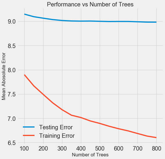
As the number of trees used by the model increases, the level of errors during training and testing decreases. But errors in training are reduced much faster, and as a result, the model is retrained: it shows excellent results on training data, but it works worse on test data.
On test data, accuracy is always reduced (after all, the model sees the correct answers for the training dataset), but a significant drop speaks of retraining . This problem can be solved by increasing the amount of training data or reducing the complexity of the model using hyper parameters . Here we will not touch on the hyperparameters, but I recommend always paying attention to the issue of retraining.
For our final model, we will take 800 appraisers, because this will give us the lowest level of error during cross-checking. Now let's test the model!
Evaluation using test data
Being responsible people, we made sure that our model did not in any way get access to test data during training. Therefore, we can use accuracy when working with test data as a quality indicator of a model when it is admitted to real problems.
We feed test data to the model and calculate the error. Here is a comparison of the results of the default gradient boost algorithm and our customized model:
# Make predictions on the test set using default and final model
default_pred = default_model.predict(X_test)
final_pred = final_model.predict(X_test)
Default model performance on the test set: MAE = 10.0118.
Final model performance on the test set: MAE = 9.0446.
Hyperparametric tuning has helped improve model accuracy by about 10%. Depending on the situation, this can be a very significant improvement, but it takes a lot of time.
You can compare the duration of training for both models using the magic command
%timeitin Jupyter Notebooks. First, measure the default duration of the model:%%timeit -n 1 -r 5
default_model.fit(X, y)
1.09 s ± 153 ms per loop (mean ± std. dev. of 5 runs, 1 loop each)One second to learn is very decent. But the tuned model is no longer so nimble:
%%timeit -n 1 -r 5
final_model.fit(X, y)
12.1 s ± 1.33 s per loop (mean ± std. dev. of 5 runs, 1 loop each)
This situation illustrates the fundamental aspect of machine learning: it’s all a matter of compromise . Constantly you have to choose a balance between accuracy and interpretability, between displacement and dispersion , between accuracy and working time, and so on. The right combination is completely determined by the specific task. In our case, the 12-fold increase in the duration of work in relative terms is large, but insignificant in absolute terms.
We obtained the final prediction results, let's now analyze them and find out if there are any noticeable deviations. On the left is a graph of the density of predicted and real values, on the right is a histogram of the error:
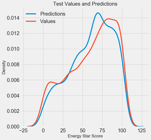

The forecast of the model reproduces well the distribution of real values, while on the training data the density peak is closer to the median value (66) than to the real peak of the density (about 100). The errors have an almost normal distribution, although there are some large negative values when the model's forecast is very different from the actual data. In the next article we will take a closer look at the interpretation of the results.
Conclusion
In this article, we looked at several stages of solving a machine learning problem:
- Filling missing values and scaling features.
- Evaluation and comparison of the results of several models.
- Hyperparameter tuning using random grid search and cross-validation.
- Evaluate the best model using test data.
The results show that we can use machine learning to predict Energy Star Score based on available statistics. With the help of gradient boosting, we managed to achieve an error of 9.1 on the test data. Hyperparameter tuning can greatly improve results, but at the cost of a significant slowdown. This is one of the many tradeoffs that need to be taken into account in machine learning.
In the next article we will try to figure out how our model works. We will also consider the main factors affecting the Energy Star Score. If we know that the model is accurate, then we will try to understand why it predicts this way and what it tells us about the task itself.