The brain from the inside (Visualization of the passage of the pattern through the model of an artificial neural network)
Introduction
The article is intended for those who have ever been interested in the question of what happens inside an artificial neural network (artificial neural network) - ANN . Now practically everyone can develop their own INS using ready-made libraries available in most programming languages. In this article, I will try to show exactly how an object ( Pattern ) looks like , passing through layers of an INS, developed and compiled using the Tensorflow deep learning library with the Keras superstructure .
Used software
The following components are necessary (the versions I have indicated for my own case):
- tensorflow 1.10.0
- keras 2.2.4
- matplotlib 2.2.0
- modul-os
- numpy1.14.3
It is also possible to draw the network architecture, but for this you need to install visualization tools, in my case keras was used , and in the method
PLOT_PATTERN_PROCCESS(...)to establish
PLOT_MODEL = True
defPLOT_PATTERN_PROCCESS(model, pattern, FOLDER_TO_SAVE, grid_size=(3, 3), limit_size_layer=(15, 15), PLOT_MODEL=True):main idea
It is necessary to choose one pattern (passage, which we will observe), after its selection the network is divided into layers of tensors . In the cycle from the second to the last layer, a new network is created, where the output is the layer number of the cycle, and skipping the pattern, the output of the network is the result in the form of an n-dimensional array.
Implementation
Connecting libraries
from keras.models import *
from keras.layers import *
import matplotlib.pyplot as plt
import os
import numpy as np
Used methods:
- def PLOT_PATTERN_PROCCESS (model, pattern, FOLDER_TO_SAVE, grid_size = (3, 3), limit_size_layer = (15, 15), PLOT_MODEL = True):
defPLOT_PATTERN_PROCCESS(model, pattern, FOLDER_TO_SAVE, grid_size=(3, 3), limit_size_layer=(15, 15), PLOT_MODEL=True):""" :param model: Модель нейроархитектуры keras :type model: Sequential :param pattern: Входной паттерн, массив данных соответвующий размеру входных слоев :type pattern: np.array :param FOLDER_TO_SAVE: Папка в которую будет сохраняться результат :type FOLDER_TO_SAVE: str :param grid_size: Размер отображаемой сетки слоев :type grid_size: tuple :param limit_size_layer: Минимальный размер для отображения слоя :type limit_size_layer: tuple :param PLOT_MODEL: Выполнить построение модели :type PLOT_MODEL: PLOT_MODEL """ SAVE_AR_LIST = [] for num_layer in range(1, len(model.layers)): LO = model.layers[num_layer].output _model = Model(inputs=model.input, outputs=LO) if ( len(_model.output_shape) == 3and _model.output_shape[1] > limit_size_layer[0] and _model.output_shape[2] > limit_size_layer[1] ): _output = _model.predict(pattern)[0] SAVE_AR_LIST.append( [ num_layer, model.layers[num_layer].name, _output.tolist() ] ) ### PIC_NUM = 0while len(SAVE_AR_LIST) > 0: fig, axs = plt.subplots(nrows=grid_size[0], ncols=grid_size[1], figsize=(10, 10), tight_layout=True) xmin, xmax = plt.xlim() ymin, ymax = plt.ylim() for ax in axs.flat: [num_layer, layer_name, ar] = SAVE_AR_LIST.pop(0) ax.imshow(np.array(ar), cmap='viridis', extent=(xmin, xmax, ymin, ymax)) ax.set_title(layer_name + " " + str(np.array(ar).shape)) if len(SAVE_AR_LIST) == 0: break# plt.show() plt.savefig(os.path.join(FOLDER_TO_SAVE, str(PIC_NUM) + '.png'), fmt='png') plt.close(fig) PIC_NUM += 1###if PLOT_MODEL: from keras.utils.vis_utils import plot_model plot_model( model=model, to_file=os.path.join(FOLDER_TO_SAVE, model.name + " neural network architecture.png"), show_shapes=True, show_layer_names=True ) ### - def build_model (IN_SHAPE = 50, CLASSES = 5) -> Sequential:
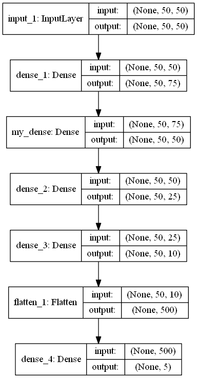
defbuild_model(IN_SHAPE=50,CLASSES=5) -> Sequential:
    inputs_LAYER0 = Input(shape=(IN_SHAPE,IN_SHAPE))
    Dense_2_2 = Dense(75, activation='relu')(inputs_LAYER0)
    Dense_2_3 = Dense(50, activation='relu', name="my_dense")(Dense_2_2)
    Dense_2_4 = Dense(25, activation='relu')(Dense_2_3)
    Dense_2_5 = Dense(10, activation='relu')(Dense_2_4)
    flat_f_0 = Flatten()(Dense_2_5)
    final_layer= Dense(CLASSES, activation='softmax')(flat_f_0)
    #
    model = Model(input=inputs_LAYER0, output=final_layer, name="simple model")
    model.compile(optimizer='adam', loss='categorical_crossentropy', metrics=['accuracy'])
    model.summary()
    return model
Program code
model_ = build_model()
pattern = np.random.sample((1,50,50))
os.makedirs("PLOT_PATTERN_PROCCESS")
PLOT_PATTERN_PROCCESS(
    model = model_,
    pattern = pattern,
    FOLDER_TO_SAVE = "PLOT_PATTERN_PROCCESS",
    PLOT_MODEL=False,
    grid_size=(2, 2)
)
Description of the program
Method
build_model()returns the ANN model in Sequential format , designed to classify something into 5 classes.
model.summary ()
_________________________________________________________________
Layer (type)                 Output Shape              Param #
=================================================================
input_1 (InputLayer)         (None, 50, 50)            0
_________________________________________________________________
dense_1 (Dense)              (None, 50, 75)            3825
_________________________________________________________________
my_dense (Dense)             (None, 50, 50)            3800
_________________________________________________________________
dense_2 (Dense)              (None, 50, 25)            1275
_________________________________________________________________
dense_3 (Dense)              (None, 50, 10)            260
_________________________________________________________________
flatten_1 (Flatten)          (None, 500)               0
_________________________________________________________________
dense_4 (Dense)              (None, 5)                 2505
=================================================================
Total params: 11,665
Trainable params: 11,665
Non-trainable params: 0
_________________________________________________________________
As can be seen from the architecture, the pattern is a 50x50 array. Variable
patternand there is an observable object.
Next, create a directory
os.makedirs("PLOT_PATTERN_PROCCESS")Where all the results will be saved.
PLOT_PATTERN_PROCCESS Method Description
I described the meaning of the method above, but it is important to say that we do not need all the layers, since the outputs of some layers cannot be displayed or it will not be informative.
Getting the output pattern occurs here:
_output = _model.predict(pattern)[0]In this implementation, you can display a two-dimensional output pattern whose dimensions are not less than the parameter
limit_size_layerAlternately, iterating over the layers of the ANN model, the variable
SAVE_AR_LIST- Layer number
num_layer - Layer name
model.layers[num_layer].name - Two-dimensional output array
_output.tolist()
Gradually eliminating one result from
SAVE_AR_LISTAnd putting it in a cell of the canvas
ax.imshow(np.array(ar), cmap='viridis', extent=(xmin, xmax, ymin, ymax))As a result, a file is created (0.png)

Recommendations
- You can set the layer name as follows:
Dense_2_3 = Dense(50, activation='relu', name="my_dense")(Dense_2_2)
This is very useful when evaluating and comparing with neuroarchitecture. - Using this approach, it is interesting to see how the pattern changes while passing the network when learning from era to era
- Do not install the grid
grid_size
large size the size of the displayed images will be small and uninformative - If you observe the passage in the dynamics (when learning or passing a pack of patterns), we are already talking about large information. To reduce the amount of RAM used by the application, it is better to save the arrays to files on a PC, for example, in JSON format , and after processing all the patterns, iterate over the files one by one and turn them into images
Successes!