Overview of graph compression algorithms
This work describes how to compress primarily social (graphs of links between users on social networks) and Web-graphs (graphs of links between sites).
Most graph algorithms are well-studied and designed with the assumption that random access to graph elements is possible. At the moment, the size of social graphs exceeds the RAM of an average machine in size, but at the same time it easily fits on a hard disk. A compromise is data compression with the ability to quickly access certain queries. We will focus on two:
a) get a list of edges for a certain vertex
b) find out if 2 vertices are connected.
Modern algorithms allow you to compress data up to 1-5 bits per link, which makes it possible to work with a similar base on an average machine. It was my desire to write this article that led me to fit the vkontakte friends database into 32GB of RAM, which, considering that there are now about 300M accounts with an average degree of top of about 100, seems quite realistic. It is on this basis that I will conduct my experiments.
The general properties of the graphs we are interested in are:
a) the fact that they are large, 1е6 - 1е9 or more vertices and of the order of 1е9 edges - which makes it impossible to work with them directly in memory, but allows them to be stored without problems even on one hard drive. The site law.di.unimi.it/datasets.php presents the entire vast range of such databases.
b) the distribution of degrees of the vertices, and indeed all important frequency characteristics are described by a power law (Power Law) at least asymptotically.
c) they are sparse. The average degree of the peak is ~ 100-1000.
d) the vertices are similar - the probability that you have a common friend is more for connected vertices.
In this paper, a graph in a “natural”, uncompressed form will be represented by an array of lists:
Table 1. Natural coding of the graph. (An example is taken from [2])
We call the difference between the indices of the two links “gap”.
The first of the families of compression algorithms are methods that use the following 2 basic approaches:
a) Operation of the locality of vertices. Peaks often refer to "close" peaks than to "distant" ones.
b) Exploitation of the similarity of vertices. “Close” peaks refer to the same peaks.
There is a paradox in these two statements - the term “proximity” of peaks can also be described through similarity, then our statements will turn into a truism. It is in explaining the concept of “proximity” that there is the main difference between the algorithms I tested.
The first work on this subject is apparently K. Randall [1]. It examined the web graph of the still surviving Altavista, and it was found that most of the links (80%) on the graph are local and have a large number of common links and it was proposed to use the following reference coding:
- the new vertex is encoded as a link to a “similar” + list additions and deletions, which in turn is encoded with gaps + nibble coding.
The guys squeezed the altavista to 5 bits per link (I will try to give the worst compression results in the works). This approach was greatly developed by Paolo Boldi and Sebastiano Vigna.
They proposed a more complex reference coding method, presented in Table 2. Each vertex can have one “similar” link, RefNr encodes the difference between the current vertex and it, if RefNr is zero, then the vertex has no link. Copy list is a bit list that encodes which vertices should be picked up by reference - if the corresponding Copy list bit is 1, then this vertex also belongs to the encoded one. Then Copylist is also encoded by RLE with a similar algorithm and turns into CopyBlocks:
We record the length - 1 for each repeating block + the value of the first block (1 or 0), and the zeros remaining at the end can be discarded.
The rest of the vertices is converted to gaps, zeros are coded separately (a special property of web graphs is used here, which will be discussed below), and the remaining gaps (Residuals) are encoded with one of the digital codes ( Golomb , Elias Gamma and as the Huffman extremum ).
As can be seen from table 2, this encoding can be multilevel - the degree of this multilevel is one of the parameters of the encoder L , with a large L, the encoding and decoding speed decreases, but the compression ratio increases.
Table 2. The method of reference coding proposed by Boldi and Vigna for the data from table 1. [2]
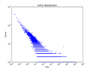
The distribution of Gaps in the crawler bases is also subject to Power-Law law.

Figure 1. The distribution of "Gaps" in snapshot on .uk sites - 18.5M pages.
That allows us to say “close” accounts are given to us from above in the form of ordered data from web crawlers. And further, we will already develop the work in the above two directions: encode the list of edges as a modification of one of the previous vertex (reference coding), store the list of edges in the form of “Gaps” (Gap [i, 0] = Node [i] - link [i, 0]) - and, using the frequency response identified above - encode this list with one of the many integer codes. I must say that they did pretty well: 2-5 bit per link [4]. In [2] and [3] even simpler reference coding methods LM and SSL were proposed which encode data in small blocks. The result is superior to or rather comparable to the BV algorithm. I want to add from myself
In social graphs - this effect does not seem to be observed - Figure 2 shows the distribution of gaps over different pieces of the vkontakte database. Interestingly, for the first million log / log accounts, the Gap Act is actually being implemented. But with an increase in the amount of data. The distribution of gaps is becoming more and more “white.”
Figure 2. Gap distribution by vkontakte friends database.
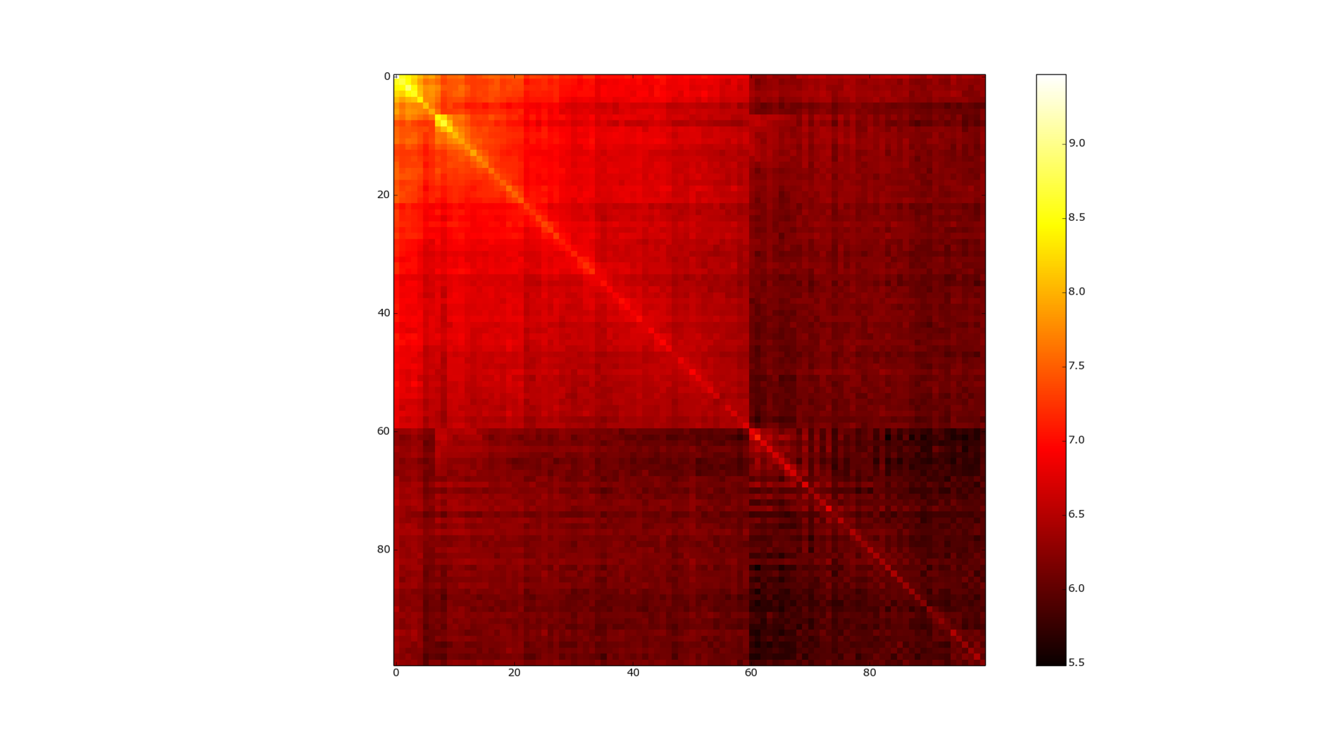
Figure 3. The adjacency matrix of the graph, vkontakte.
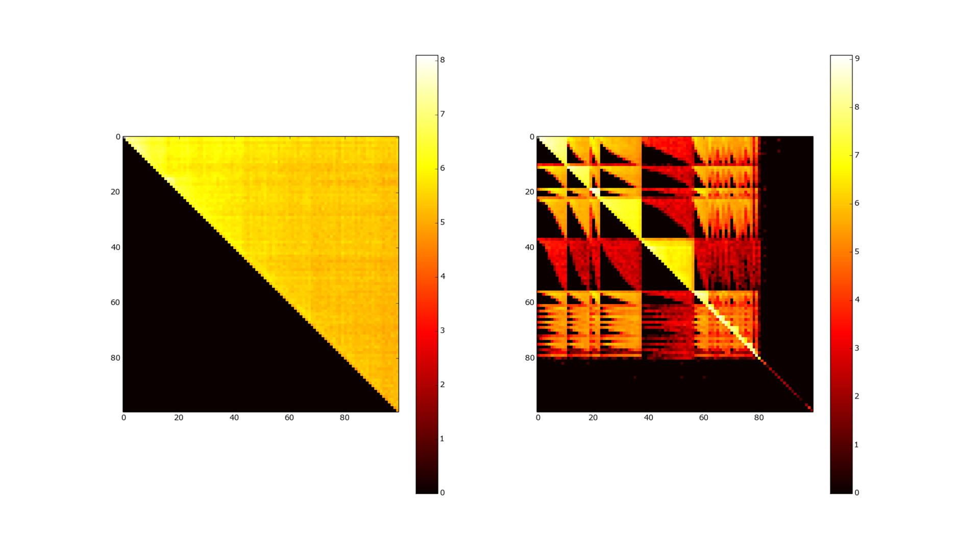
Figure 4. Adjacency matrix before and after clustering. 100k users.
Figure 3 shows the adjacency matrix of the friends graph, in a logarithmic form. She also does not inspire much hope for this kind of compression. The data looks much more interesting if you somehow cluster our graph in advance. Figure 4 shows the adjacency matrix after passing the MCL ( Markov Cluster Algorithm) clustering. The correspondence matrix becomes almost diagonal (the color map is logarithmic, so bright yellow means several orders of magnitude more connections between elements) - and WebGraph and many other algorithms are already great for compressing such data. (Asano [7] is currently the best as far as I know from compression, but also the slowest in access to data).
But the problem is that the MCL in the worst case is cubic in time and quadratic in memory (http://micans.org/mcl/man/mclfaq.html#howfast). In life, everything is not so bad for symmetric graphs (which a social graph is almost) - but it is all the same far from linearity. An even bigger problem is that the graph does not fit in memory and you need to come up with distributed clustering techniques - and this is a completely different story. An intermediate solution to this problem was invented by Alberto Apostolico and Guido Drovandi [1] - renumbering a graph by simply going through it with a breadth-first search (BFS-search). Thus, it is guaranteed that some of the nodes referring to each other will have close indices. In their work, they left GAP coding and replaced it with a rather complex model of reference coding, having received 1-3 bits per encoded link. Actually, the intuition by which BFS should correctly compose the vertices is not very clear, but this method works - I did this coding for the VKontakte database and looked at the histogram by the gaps (Figure 5) - it looks very promising. There are also suggestions to use Deep First Search instead of BFS, as well as more complex reindexing schemes such as shingle reordering [7] - they give a similar increase. There is one more reason why BFS reindexing should / can work - WebArchive databases are well-encoded, and they are obtained just by sequential indexing of a live Internet graph. There are also suggestions to use Deep First Search instead of BFS, as well as more complex reindexing schemes such as shingle reordering [7] - they give a similar increase. There is one more reason why BFS reindexing should / can work - WebArchive databases are well-encoded, and they are obtained just by sequential indexing of a live Internet graph. There are also suggestions to use Deep First Search instead of BFS, as well as more complex reindexing schemes such as shingle reordering [7] - they give a similar increase. There is one more reason why BFS reindexing should / can work - WebArchive databases are well-encoded, and they are obtained just by sequential indexing of a live Internet graph.
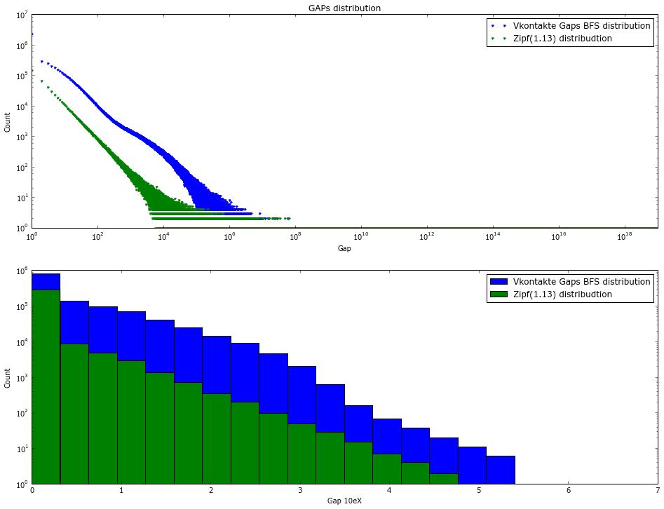
Figure 5. Gap distribution by vkontakte friends database after BFS indexing. 100k sampling
Table 2. Gap distribution by vkontakte friends database after BFS indexing. 1M sample
The second work of Boldi and Vigna [5] is devoted to the theoretical justification of coding the list of gaps with various digital codes, as well as comparing them with Huffman coding as possible upper bound. The basis is the fact that the encoded value is distributed according to the Zipf law. The upper compression limit for various alpha parameters turned out to be 4-13 bits per link. For the VKontakte database, this encoding method gave 18 bits per link. Which, of course, is no longer bad and allows you to fit the entire base in RAM, but it is very far from the territorial estimates given in the works. Figure 5 shows a comparison of the distribution of gaps after BFS indexation, with the distribution of the zipf as close as possible to practical data (alpha = 1.15). Figure 6 shows the adjacency matrix for the graph after BFS reindexing - it displays the reason for poor compression well - the diagonal is well drawn but the overall noise is still very large compared to the clustered matrix. These “bad” results are also confirmed by work [6].
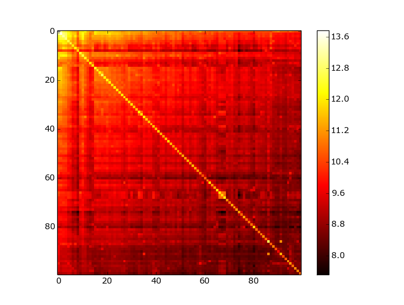
Figure 6. Adjacency matrix of vkontakte base. After BFS reindexing.
There is another method that deserves special attention - exploitation of graph properties. Namely, the selection of a bipartite graph and the generation of a virtual vertex connecting the 2 parts of the subgraph. This reduces the length of the vertex lists for each side of the bipartite graph. This task is generally NP-complete, but there are many good heuristics for finding bipartite subgraphs. This method was proposed in [9], just like the BV algorithm spawned many others [10–11] and deserves a more detailed consideration. Figure 6 describes only his main idea.
Figure 6. Biklik coding.
Most graph algorithms are well-studied and designed with the assumption that random access to graph elements is possible. At the moment, the size of social graphs exceeds the RAM of an average machine in size, but at the same time it easily fits on a hard disk. A compromise is data compression with the ability to quickly access certain queries. We will focus on two:
a) get a list of edges for a certain vertex
b) find out if 2 vertices are connected.
Modern algorithms allow you to compress data up to 1-5 bits per link, which makes it possible to work with a similar base on an average machine. It was my desire to write this article that led me to fit the vkontakte friends database into 32GB of RAM, which, considering that there are now about 300M accounts with an average degree of top of about 100, seems quite realistic. It is on this basis that I will conduct my experiments.
The general properties of the graphs we are interested in are:
a) the fact that they are large, 1е6 - 1е9 or more vertices and of the order of 1е9 edges - which makes it impossible to work with them directly in memory, but allows them to be stored without problems even on one hard drive. The site law.di.unimi.it/datasets.php presents the entire vast range of such databases.
b) the distribution of degrees of the vertices, and indeed all important frequency characteristics are described by a power law (Power Law) at least asymptotically.
c) they are sparse. The average degree of the peak is ~ 100-1000.
d) the vertices are similar - the probability that you have a common friend is more for connected vertices.
Boldi and Vigna.
In this paper, a graph in a “natural”, uncompressed form will be represented by an array of lists:
node1 -> link11,link12,link13...
node2 -> link21,link22,link23....
....
Где link[i,j] < link[i,j+1].
| Vertex | Vertex degree | Ribs |
|---|---|---|
| fifteen | eleven | 13,15,16,17,18,19,23,24,203,315,1034 |
| 16 | 10 | 15,16,17,22,23,24,315,316,317,3041 |
| 17 | 0 | |
| 18 | 5 | 13,15,16,17,50 |
Table 1. Natural coding of the graph. (An example is taken from [2])
We call the difference between the indices of the two links “gap”.
Gap[i,j] = link[i,j-1] - link[i,j] The first of the families of compression algorithms are methods that use the following 2 basic approaches:
a) Operation of the locality of vertices. Peaks often refer to "close" peaks than to "distant" ones.
b) Exploitation of the similarity of vertices. “Close” peaks refer to the same peaks.
There is a paradox in these two statements - the term “proximity” of peaks can also be described through similarity, then our statements will turn into a truism. It is in explaining the concept of “proximity” that there is the main difference between the algorithms I tested.
The first work on this subject is apparently K. Randall [1]. It examined the web graph of the still surviving Altavista, and it was found that most of the links (80%) on the graph are local and have a large number of common links and it was proposed to use the following reference coding:
- the new vertex is encoded as a link to a “similar” + list additions and deletions, which in turn is encoded with gaps + nibble coding.
The guys squeezed the altavista to 5 bits per link (I will try to give the worst compression results in the works). This approach was greatly developed by Paolo Boldi and Sebastiano Vigna.
They proposed a more complex reference coding method, presented in Table 2. Each vertex can have one “similar” link, RefNr encodes the difference between the current vertex and it, if RefNr is zero, then the vertex has no link. Copy list is a bit list that encodes which vertices should be picked up by reference - if the corresponding Copy list bit is 1, then this vertex also belongs to the encoded one. Then Copylist is also encoded by RLE with a similar algorithm and turns into CopyBlocks:
01110011010 -> 0,0,2,1,1,0,0
We record the length - 1 for each repeating block + the value of the first block (1 or 0), and the zeros remaining at the end can be discarded.
The rest of the vertices is converted to gaps, zeros are coded separately (a special property of web graphs is used here, which will be discussed below), and the remaining gaps (Residuals) are encoded with one of the digital codes ( Golomb , Elias Gamma and as the Huffman extremum ).
As can be seen from table 2, this encoding can be multilevel - the degree of this multilevel is one of the parameters of the encoder L , with a large L, the encoding and decoding speed decreases, but the compression ratio increases.
| Vertex | Vertex degree | RefNr | number of copy blocks | Copy blocks | Number of intervals | intervals (relative left index) | interval lengths | Residual |
|---|---|---|---|---|---|---|---|---|
| ... | ... | ... | ... | ... | ... | ... | ... | ... |
| fifteen | eleven | 0 | 2 | 0.2 | 3.0 | 5,189,11,718 | ||
| 16 | 10 | 1 | 7 | 0,0,2,1,1,0,0 | 1 | 600 | 0 | 12,3018 |
| 17 | 0 | |||||||
| 18 | 5 | 3 | 1 | 4 | 0 | fifty | ||
| ... | ... | ... | ... | ... | ... | ... | ... | ... |
Table 2. The method of reference coding proposed by Boldi and Vigna for the data from table 1. [2]
The distribution of Gaps in the crawler bases is also subject to Power-Law law.

Figure 1. The distribution of "Gaps" in snapshot on .uk sites - 18.5M pages.
That allows us to say “close” accounts are given to us from above in the form of ordered data from web crawlers. And further, we will already develop the work in the above two directions: encode the list of edges as a modification of one of the previous vertex (reference coding), store the list of edges in the form of “Gaps” (Gap [i, 0] = Node [i] - link [i, 0]) - and, using the frequency response identified above - encode this list with one of the many integer codes. I must say that they did pretty well: 2-5 bit per link [4]. In [2] and [3] even simpler reference coding methods LM and SSL were proposed which encode data in small blocks. The result is superior to or rather comparable to the BV algorithm. I want to add from myself
In social graphs - this effect does not seem to be observed - Figure 2 shows the distribution of gaps over different pieces of the vkontakte database. Interestingly, for the first million log / log accounts, the Gap Act is actually being implemented. But with an increase in the amount of data. The distribution of gaps is becoming more and more “white.”
 | 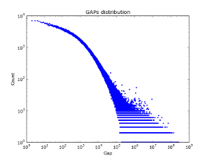 | 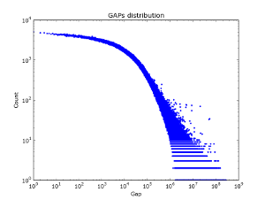 |
| Sample 50k. | 100k sample | 2M sample. |
Figure 2. Gap distribution by vkontakte friends database.

Figure 3. The adjacency matrix of the graph, vkontakte.

Figure 4. Adjacency matrix before and after clustering. 100k users.
Figure 3 shows the adjacency matrix of the friends graph, in a logarithmic form. She also does not inspire much hope for this kind of compression. The data looks much more interesting if you somehow cluster our graph in advance. Figure 4 shows the adjacency matrix after passing the MCL ( Markov Cluster Algorithm) clustering. The correspondence matrix becomes almost diagonal (the color map is logarithmic, so bright yellow means several orders of magnitude more connections between elements) - and WebGraph and many other algorithms are already great for compressing such data. (Asano [7] is currently the best as far as I know from compression, but also the slowest in access to data).
But the problem is that the MCL in the worst case is cubic in time and quadratic in memory (http://micans.org/mcl/man/mclfaq.html#howfast). In life, everything is not so bad for symmetric graphs (which a social graph is almost) - but it is all the same far from linearity. An even bigger problem is that the graph does not fit in memory and you need to come up with distributed clustering techniques - and this is a completely different story. An intermediate solution to this problem was invented by Alberto Apostolico and Guido Drovandi [1] - renumbering a graph by simply going through it with a breadth-first search (BFS-search). Thus, it is guaranteed that some of the nodes referring to each other will have close indices. In their work, they left GAP coding and replaced it with a rather complex model of reference coding, having received 1-3 bits per encoded link. Actually, the intuition by which BFS should correctly compose the vertices is not very clear, but this method works - I did this coding for the VKontakte database and looked at the histogram by the gaps (Figure 5) - it looks very promising. There are also suggestions to use Deep First Search instead of BFS, as well as more complex reindexing schemes such as shingle reordering [7] - they give a similar increase. There is one more reason why BFS reindexing should / can work - WebArchive databases are well-encoded, and they are obtained just by sequential indexing of a live Internet graph. There are also suggestions to use Deep First Search instead of BFS, as well as more complex reindexing schemes such as shingle reordering [7] - they give a similar increase. There is one more reason why BFS reindexing should / can work - WebArchive databases are well-encoded, and they are obtained just by sequential indexing of a live Internet graph. There are also suggestions to use Deep First Search instead of BFS, as well as more complex reindexing schemes such as shingle reordering [7] - they give a similar increase. There is one more reason why BFS reindexing should / can work - WebArchive databases are well-encoded, and they are obtained just by sequential indexing of a live Internet graph.

Figure 5. Gap distribution by vkontakte friends database after BFS indexing. 100k sampling
| Gap | number | Share |
|---|---|---|
| 1 | 83812263 | 7.69% |
| 2 | 12872795 | 1.18% |
| 3 | 10643810 | 0.98% |
| 4 | 9097025 | 0.83% |
| 5 | 7938058 | 0.73% |
| 6 | 7032620 | 0.65% |
| 7 | 6322451 | 0.58% |
| 8 | 5733866 | 0.53% |
| 9 | 5230160 | 0.48% |
| 10 | 4837242 | 0.44% |
| top10 | 153520290 | 14.09% |
Table 2. Gap distribution by vkontakte friends database after BFS indexing. 1M sample
The second work of Boldi and Vigna [5] is devoted to the theoretical justification of coding the list of gaps with various digital codes, as well as comparing them with Huffman coding as possible upper bound. The basis is the fact that the encoded value is distributed according to the Zipf law. The upper compression limit for various alpha parameters turned out to be 4-13 bits per link. For the VKontakte database, this encoding method gave 18 bits per link. Which, of course, is no longer bad and allows you to fit the entire base in RAM, but it is very far from the territorial estimates given in the works. Figure 5 shows a comparison of the distribution of gaps after BFS indexation, with the distribution of the zipf as close as possible to practical data (alpha = 1.15). Figure 6 shows the adjacency matrix for the graph after BFS reindexing - it displays the reason for poor compression well - the diagonal is well drawn but the overall noise is still very large compared to the clustered matrix. These “bad” results are also confirmed by work [6].

Figure 6. Adjacency matrix of vkontakte base. After BFS reindexing.
Biklik
There is another method that deserves special attention - exploitation of graph properties. Namely, the selection of a bipartite graph and the generation of a virtual vertex connecting the 2 parts of the subgraph. This reduces the length of the vertex lists for each side of the bipartite graph. This task is generally NP-complete, but there are many good heuristics for finding bipartite subgraphs. This method was proposed in [9], just like the BV algorithm spawned many others [10–11] and deserves a more detailed consideration. Figure 6 describes only his main idea.
 | 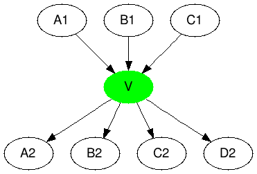 |
| A1 -> A2 B2 C2 D3 B1 -> A2 B2 C2 D4 C1 -> A2 B2 C2 D5 | A1 -> V D3 B1 -> V D4 C1 -> V D5 V -> A2 B2 C2 |
Figure 6. Biklik coding.
Literature
- A. Alberto and G. Drovandi: Graph compression by BFS.
- Sz. Grabowski and W. Bieniecki: Tight and simple Web graph compression.
- Sz. Grabowski and W. Bieniecki Merging adjacency lists for efficient Web graph compression
- P. Boldi and S. Vigna: The webgraph framework I: Compression techniques.
- P. Boldi and S. Vigna: The webgraph framework II: Codes for the World-Wide-Web. WebGraphII.pdf
- P. Boldi and S. Vigna. Permuting Web and Social Graphs.
- Flavio Chierichetti, Ravi Kumar. On Compressing Social Networks.
- Y. Asano, Y. Miyawaki, and T. Nishizeki: Efficient compression of web graphs.
- Gregory Buehrer, Kumar Chellapilla. A Scalable Pattern Mining Approach to Web Graph Compression with Communities
- Cecilia Hernandez, Gonzalo Navarro. Compressed Representations for Web and Social Graphs.
- F. Claude and G. Navarro: Fast and compact web graph representations.