2GIS user statistics: ETL rules and data preprocessing

In order to understand user preferences and evaluate the performance of 2GIS services, we collect anonymized information. Our customers are product managers, representatives of commerce and marketing, partners and advertisers who view statistics in their personal dashboard.

User statistics has from 21 to 27 parameters. It includes a city, a heading, a company, and so on.

A large number of event parameters leads to a large number of reports: total indicators, average values, deviations, top-10, -100, -1000 and much more. In this scenario, it is difficult to predict what kind of information will come in handy tomorrow. And when this need arises, it will be necessary to provide data as soon as possible.

Is that familiar?

In numbers

26 million users of 2GIS form about 200 million events per day. These are approximately 2400 rps that need to be received, processed and saved. The data obtained must be optimized for arbitrary ad hoc and analytical queries.

The challenge is:
- Prepare data (ETL). This is the most significant and time-consuming step.
- Calculate aggregates (preprocessing).

To begin, we will solve the first question.

As it was before

Once upon a time, our business intelligence system looked completely different. It was perfect for working with a small number of cities, but when we entered new markets, this system was cumbersome and inconvenient:

1. Data was stored in non-partitioned tables and updated with the standard “insert” and “update”. Operations applied to the entire data array.
2. With new requests for data, tables were overgrown with indices, which:
   a) had to be rebuilt when new data was received;
   b) occupied more and more space.
3. The join operations of multi-million tables were almost impossible.
4. Administrative operations — backup, compression, and index rebuilding — took a long time.
5. To process a multidimensional database, I had to process the entire data array daily. Even those that have not changed.
6. Analytical queries on a multidimensional database also took a lot of time.

Therefore, we decided to process the data differently.

New approach

Partitioning + files + filegroups

Partitioning is the presentation of a table as a single logical entity, while its parts - sections - can physically reside in different files and file groups.

The table is partitioned using the partition function. It defines the range boundaries for the values ​​of the partitioning column. Based on the partition function, a partition scheme is constructed. The choice of the partition function is key because profit in queries for data retrieval will be only if a partitioning column is used in the query. In this case, the partitioning scheme will indicate where to look for the required data.



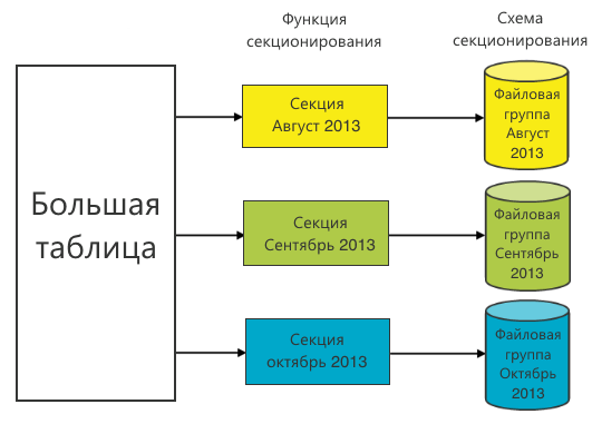
Often, the time (day, month, year) is selected as a partition function. This is due to the historicity of the data: old data does not change. This means that the sections in which they are located can be placed in file groups and accessed only as necessary in the old periods. To save resources, they can even be put on slow drives.

We chose the month as the partition function, because most queries are built on a monthly basis.



However, there are several problems.

1. Paste is still happening in a large table. If it has an index, then inserting new data will lead to a rebuild of the index, and an increase in the number of indices will inevitably slow down the operation of inserting new data.
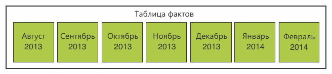
2. For partitioning multidimensional databases, Microsoft recommends using sections of up to 20 million records. Our sections turned out to be an order of magnitude larger. This threatened us with performance gaps in the preprocessing phase. Uncontrolled growth in section size could negate the whole idea of ​​sectioning.

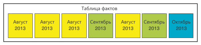
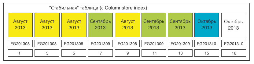
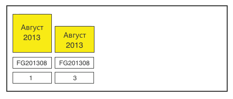
To solve the second question, we increased the number of sections for each period. If we use the month and a certain serial number of the section of this month as the partition function, we get the following.



The first problem was more difficult. We dealt with it, but to evaluate our solution, you need to know about the Columnstore index.

Columnstore index

In fairness, it is worth saying that the Columnstore index is not an index in the classical sense. It works differently .

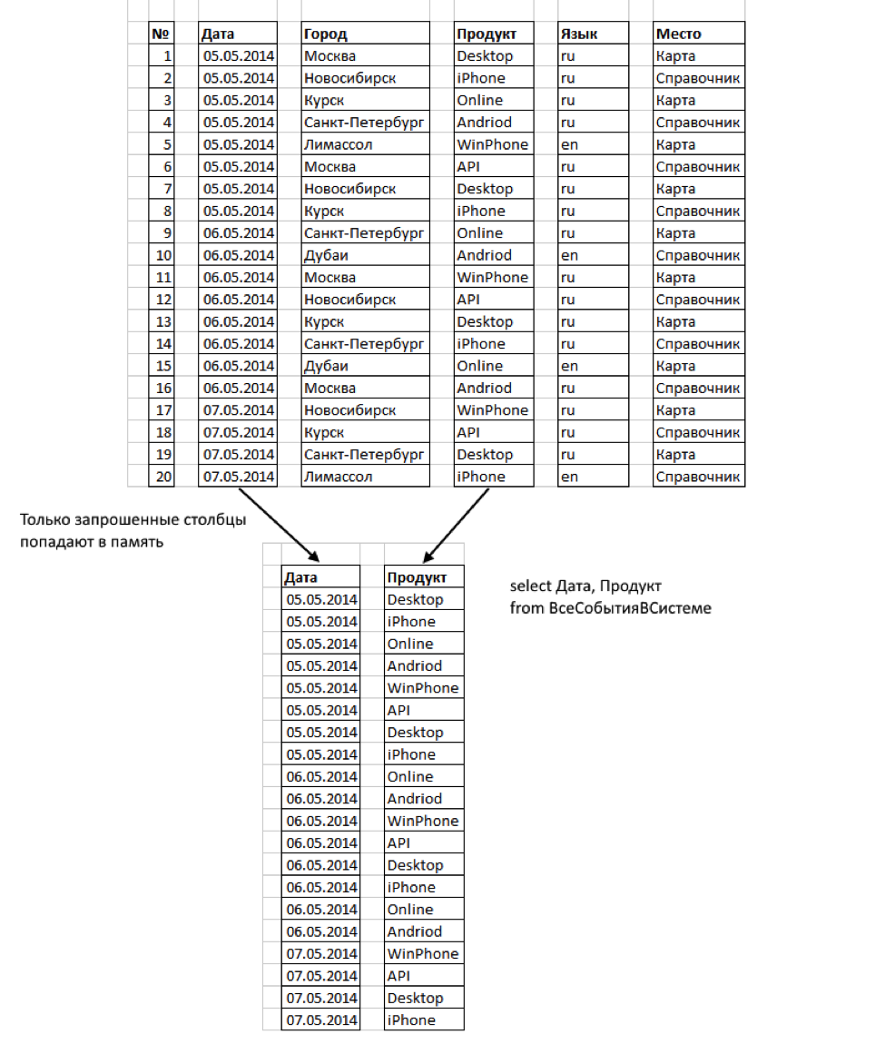
Starting from version 2012, MS SQL Server supports Columnstore - storing data in columns. Unlike the usual storage of data in rows, the information there is grouped and stored 1 column at a time.

This format has several advantages:

- Only those columns that we request are read. Some columns may never be remembered at all.
- The columns are very compressed. This reduces the bytes to be read.
- The concept of key columns does not exist in the Columnstore index. The limit on the number of key columns in an index (16) does not apply to Columnstore indexes. In our case, this is important, because the number of parameters (Rowstore columns) is much greater than 16.
- Columnstore indexes work with partitioning tables. Columnstore on a partitioned table should be aligned in sections with the base table. Thus, a nonclustered Columnstore index can be created for a partitioned table only if the partitioning column is one of the columns in that index. This is not a problem for us, because Partitioning is done on time.



“Great!” We thought. “That's what you need.” However, one feature of the Columnstore index turned out to be a problem: in SQL Server 2012, a table with a Columnstore index cannot be updated. The operations "insert", "update", "delete" and "merge" are not allowed.

The option of deleting and rebuilding the index for each data insert operation turned out to be inapplicable. Therefore, we solved the problem by switching sections.

Section Switching

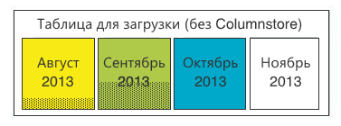
Let's go back to our table. Now she is with the Columnstore index.



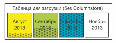
Let's create one more table with the following properties:

- all the same columns and data types;
- the same sectioning, only 1 section for each month;
- without Columnstore index.



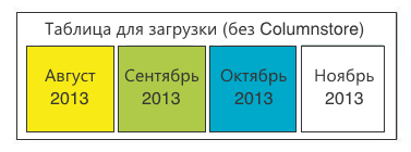
We upload new data into it: we will transfer sections from there to a stable table.

Go.

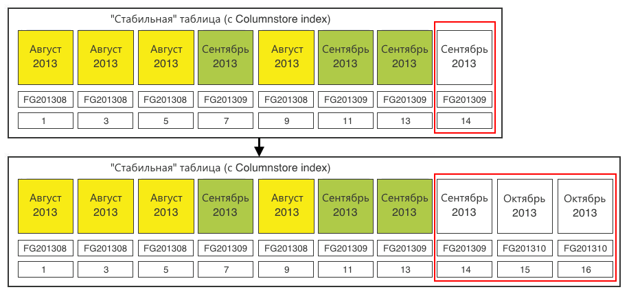
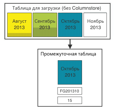
Step 1. We determine the sections that require switching. We need sections of 20 million records. We load the data and at a certain iteration we find that one of the sections is full.



Step 2In a stable table, create a section for switchable data. The section must be created in the corresponding file group - October 2013. The existing empty section (14) in the September file group does not suit us. We create section (15) for loading data there. Plus, we make one extra section (16), which we will “propagate” the next time, because always to propagate, you need one empty section at the end.



Step 3. Switch the destination section to the staging table.



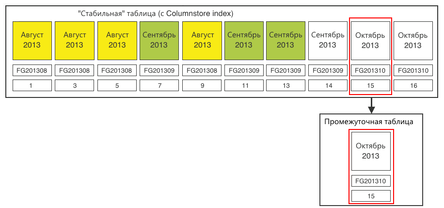
Step 4. Fill the data from the table to load the data into the intermediate table. After that, you can create a Columnstore index on the staging table. For 20 million records, this is done very quickly.



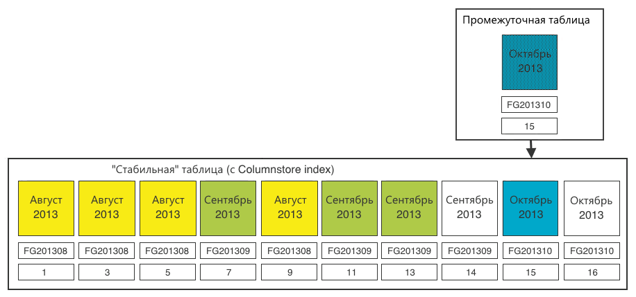
Step 5. Switch the section from the staging table to the stable one.

Now:

- columns and data types are the same;
- a new section in the file group corresponding to this section;
- We have already created the Columnstore index in the new section, and it fully corresponds to the index of the stable table.



Step 6. For complete cleanliness, close the empty (14) section in the stable table that we no longer need.



Bottom line - the table for downloading is again ready to receive data.



The stable table was replenished with one section (15). The last section (16) is ready for reproduction identical to step 2.



In general, the task has been achieved. From here you can proceed to the preprocessing (preliminary preparation) of the data.

Multidimensional Database Processing (OLAP)

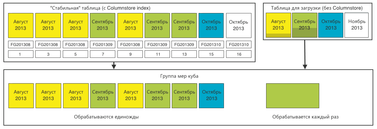
Let me remind you: we need to provide online data analysis for an arbitrary set of columns with arbitrary filtering, grouping and sorting. To do this, we decided to use the multidimensional OLAP database, which also supports partitioning.

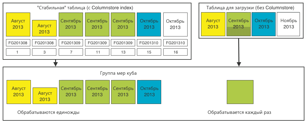
We create sections identical to our tables. Only for the main “stable” table we cut the 1-in-1 sections according to the relational database.
And for the loading table, one common section is enough.

Now we have got calculated units (sums) for the Cartesian product of all parameters in each section. During a user query, a multidimensional database will read the sections corresponding to the query and sum the aggregates among themselves.

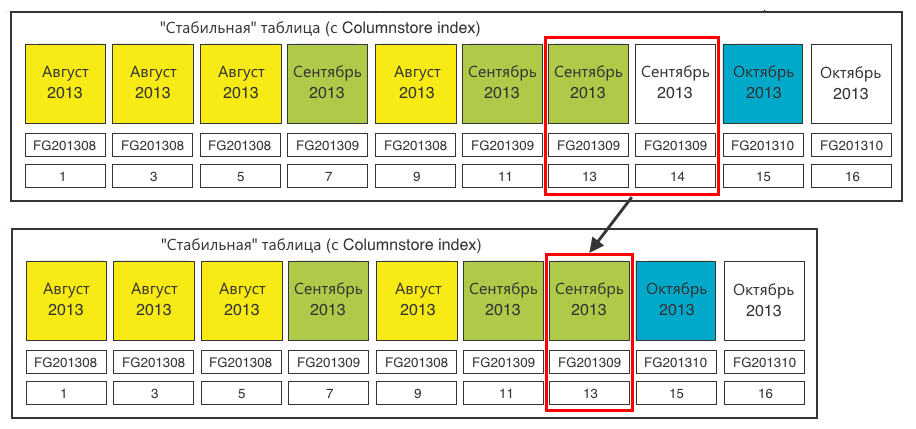
Compression of old periods

So, we did everything as described above, but found that the same month was spread over a significant number of sections. At the same time, the number of sections for each month increases with the number of users, cities of coverage, platforms, etc.

This monthly increases the time it takes to prepare a report. Yes, and just - takes up extra disk space.

We analyzed the contents of the sections of one month and came to the conclusion that we can compress it by aggregating over all significant fields. Detailing in time turned out to be enough for us up to date. Compression of old periods is especially effective when historical data is no longer being received and the number of sections for compression is maximum.

How we did it:

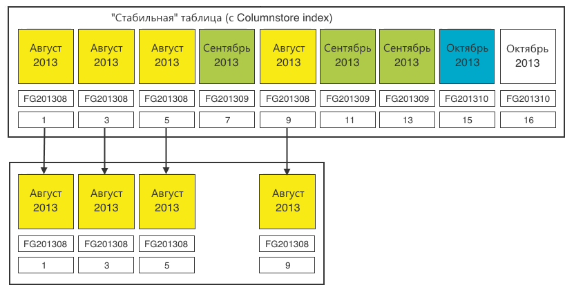
Step 1. We define all sections of one month.



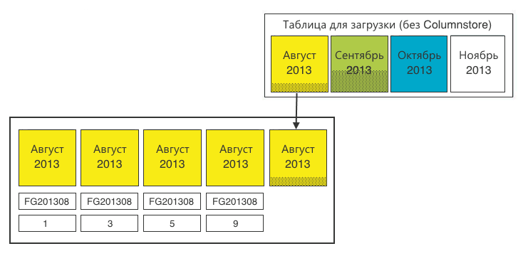
Step 2Add the leftovers from the loading table.



Step 3. Aggregate over all relevant fields. The operation is performed approximately once a month, so here it is quite possible to donate resources.

At this stage, it may turn out that the size of the sections obtained does not correspond to our ideal 20 million. There is nothing to be done about it. At the very least, the fact that the last section of each month will be incomplete does not affect performance in any way.



Step 4. In the end, do not forget to redraw the multidimensional database. Full processing takes about 5-6 hours. This is perfectly acceptable for a monthly operation.

Summary

Partitioning for large tables is a must have

Partitioning allows you to spread the load across files, filegroups and disks. Moreover, even with the use of sectioning, size matters.

We set ourselves the goal of forming 20 million sections in order to use them in the future to build a multidimensional database. In each case, the size of the section should be determined by the problem being solved.

The partitioning function is also critical.

Columnstore index decides!

We have covered all ad hoc requests. We do not need to create / rebuild indexes when new tasks for data sampling appear.

The implementation of the Columnstore index in MS SQL Server 2012 actually duplicates the original Rowdata table, creating the same, but with column storage.

Nevertheless, the amount of data occupied by the index is much smaller than if we created a set of special indexes for each task.

The insert constraint is bypassed by switching sections.

Results in numbers

For example, one of the tables: 3,940,403,086 rows; 285 887,039 MB

Request Execution Time	Partitioned table	Partitioned Table + Columnstore	Multidimensional OLAP Database
The number of calls on May 5 from the iPhone version in Moscow	8 minutes 3 sec	7 sec	6 sec
Physical size of type A events	285.9 GB	285.9 GB + 0.7 GB index	67 GB

What other options are there?

Not MS

Historically, all enterprise development in the company is based on Microsoft solutions. We went the same way and did not consider other options in principle. Fortunately, MS SQL Server supports working with large tables at all levels of processing. These include:

- Relational database (Data Warehousing);
- Sql Server Integration Services (ETL);
- Sql Server Analysis Services (OLAP).

MS SQL Server 2014

In SQL Server 2014, Columnstore functionality was expanded to become clustered . Newly received data falls into Deltastore - traditional (Rowstore) data storage, which switches to the main Columnstore as it accumulates.
If you don’t need to clearly size the partitions, SQL Server 2014 is a great solution for collecting, processing, and analyzing user statistics.