Hedgehog in fractal fog

This article is the last of a series of my hairstyles about fractals. In habrastatia “We draw pictures using the Hilbert curve”, we talked about a kitten named Gav, in habrastatia “Kosh on the complex plane” - about flowing fractals into the horizon, in habrastatia “Night of fractals” - about the runaway time algorithm. This article will discuss the hedgehog in the fog and, of course, the cat.





Everyone who even at least slightly encountered fractals saw beautiful pictures of Julia sets defined by a square polynomial; but it is interesting to solve the inverse problem: let there be some picture, and we go along it to come up with such a polynomial that will give some approximation of the original picture. The picture with the hedgehog above demonstrates this idea.

So, consider the cat the K .



We need to come up with a polynomial f such that inside the cat the sequence f ( z ), f ( f ( z )), f ( f ( f ( z ))), ... is bounded, and outside the cat it tends to infinity. I did not think about this question for a long time, but immediately searched the Internet and found a wonderful article by Kathryn A. Lindsey , “Shapes of polynomial Julia sets” , 2013, arXiv: 1209.0143 . This article proves that for "good"cat and for a given accuracy δ such a polynomial can be invented, and the proof is constructive.

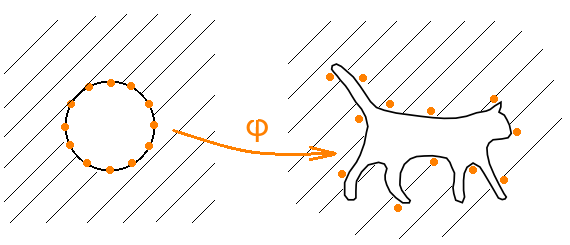
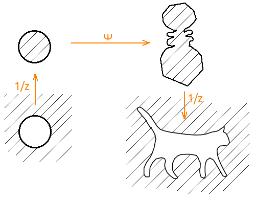
Consider this design. Let φ 'be a conformal mapping that transforms the exterior of the unit circle into the exterior of the cat. Let φ ( z ) = φ '((1 + ε) z ) be the original map corrected for some small ε.



Further, let ω ( z ) = c ^{- n} ( z - r ₀ ) ( z - r ₁ ) ⋅ ... ⋅ ( z - r _{n −1} ), where c is the coefficient of zmapping φ expansion in a Laurent series, and r _k = φ (e ^{2π ik / n} ) - images roots of unity n -th degree. It is proved that the polynomial f ( z ) = z (ω ( z ) + 1) is the desired one for sufficiently large n .

Therefore, to solve our problem, we must learn to generate the corresponding conformal mapping. As a result of a small search on the Internet, a zipper package was found . This package allows you to find a conformal mapping of the interior of a unit circle onto a region bounded by a polyline. Although this package was written twenty years agoin ancient dialect , it was not difficult to assemble it and use it.



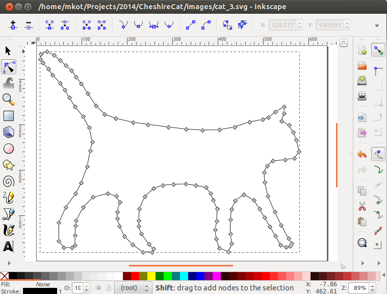
To use this package, you need to build a polyline on the image. I didn’t make any automatic decisions, but uploaded the image to the Inkscape editor and circled it, and it was easy to parse the SVG format. This is convenient because it allows you to experiment with a polyline.




Next, we need a mapping from the exterior to the exterior, and the package finds the mapping from the inside to the inside. Here you just need to pair the generated display with inversion. That is, φ '( z ) = 1 / ψ (1 / z ), where ψ is the map that generates the packet. And the input of the packet must be submitted already inverted broken.




The coefficient c is still involved in the definition of the polynomial f . For an approximate calculation of its value, we use the following trick. Let f ( z ) = c z + a + a ₁ / z + a ₂ / z ² + a ₃ / z ³ + ... Consider some finite, but rather large, part of this series. We substitute the values of a number of roots of unity of n -th degree, where n greater than the number of members of this piece. f (e <sup>2π





ik / n</sup> ) = c e ^{2π ik / n} + a + a ₁ e ^{−2π ik / n} + a ₂ e ^{−4π ik / n} + a ₃ e ^{−6π ik / n} + ..., k = 0 ^,. .., n - 1.

Now multiply each line by e ^{−2π ik / n} and add all the lines. Since the sum of all roots of unity is 0, only n c remains on the right. Therefore, we can put

c = ( f (1) ⋅ 1 + f (e ^{2π i / n} ) e ^{−2π i / n} + ... + f (e ^{2π i ( n - 1) / n} ) e ^{−2π i ( n - 1) / n} )) / n .

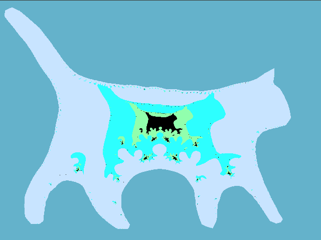
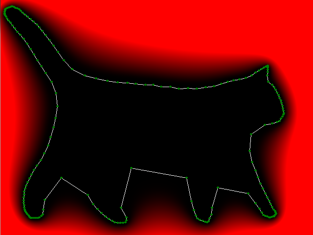
Put it all together and check what happened. The figure below shows the "thermal" graph of the logarithm of the module f ( z) (the redder, the greater the value). As you can see, inside the cat the values ​​of the polynomial are small, and outside the cat the polynomial increases, it should be so. Notice also how the f (e ^{2π ik / n} ) values ​​are distributed (green dots), because of this effect, we had to draw a cat whose legs are far enough apart.



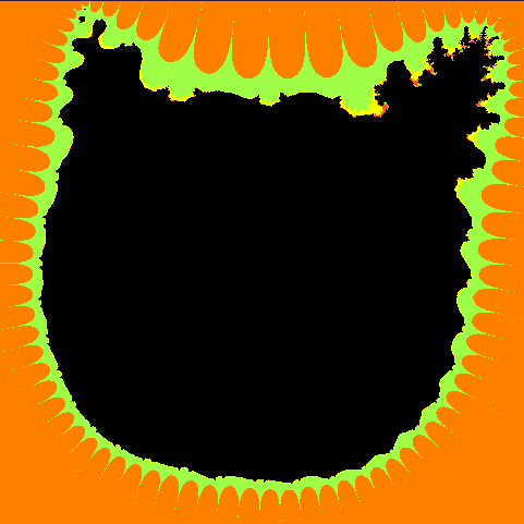
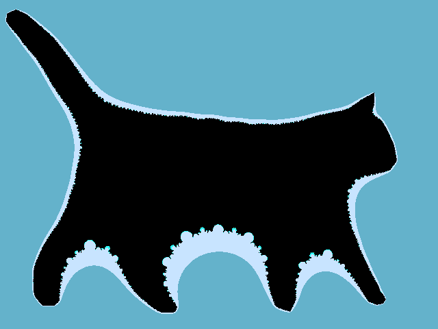
Now we simply use some algorithm to draw the Julia set and get a cat whose border is fractal.




If our image consists of several regions A ₁ , A ₂ , ..., A _q , then in the above article it is proposed to use instead of the polynomial the rational map f ( z ) defined as follows. For each region A _r , we write the product ω _r ( z ) as done above. Then the desired rational function f ( z ) is determined by the formula f ( z ) = z / (1 / ω ₁ ( z ) + ... + 1 / ω _q (z )).

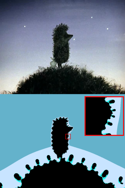
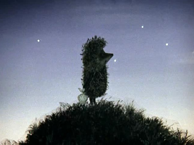
For example, let us have a hedgehog in the fog of Ye .



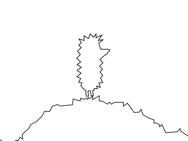
Circle the hedgehog and the hill (the lower border of the hill is outside the picture).



Hedgehog in a vacuum.



Hill without a hedgehog.



Together.



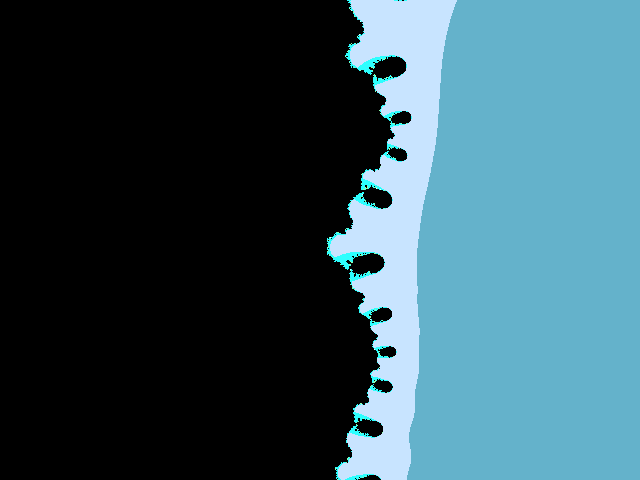
Enlarged hedgehog belly with hedgehog fleas.



As always, the source code can be found on the github .

Once again, I’ll repeat the link to the article with which everything turned out: Kathryn A. Lindsey , “Shapes of polynomial Julia sets” , 2013, arXiv: 1209.0143 . I note that the article is easy to read, so you can sort the evidence over a cup of tea.

I hope it was fun.