Atmospheric absorption or how to assess air pollution
Many here are fond of astrophotography and for the mighty it has become a favorite pastime. However, you can find a very interesting application for your hobby and do a whole study on the basis of one photograph. Today we will try to estimate the degree of air pollution in your city from a photograph. Anyone interested in the post, then welcome to cat.
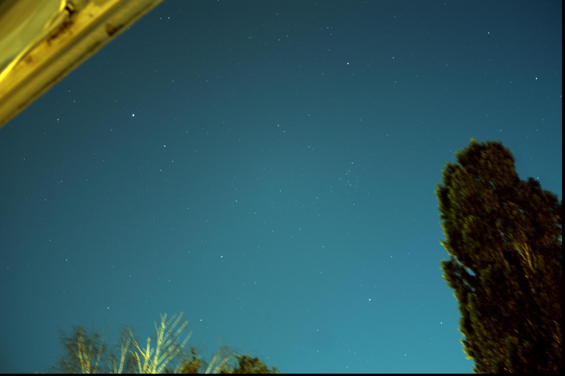
Our atmosphere is not perfectly transparent: in addition to air there are gas and dust that get there in different ways, in cities, as a rule, due to industrial enterprises or car exhausts. Due to all this, the radiation that passes through the atmosphere is significantly attenuated. And the longer the path that light travels in the atmosphere, the stronger this attenuation. If you look at the figure below, it turns out that the path in the atmosphere is the longer, the lower the height of the light source:

Let's try to derive the dependence of the long path of a light beam in the atmosphere on the height of the light source:

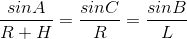
We apply the sine theorem to this triangle:
Using the fact that A = 90 + h, where h is the height of the star, we get:
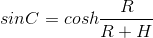
Further, using the first and last relation from the sine theorem, as well as the theorem on the sum of the angles in a triangle, we get:

Here we used the following:

However, the path length in the atmosphere is usually expressed not in dimension of length, but in dimensionless expressions, i.e. length The paths of a ray of light in the atmosphere are expressed in the heights of a homogeneous atmosphere, and such a unit is called the atmospheric mass (eng: airmass). Let k = R / H be the ratio of the radius of the Earth and the height of a homogeneous atmosphere (k = 800)
Then in the air masses our formula will take the form:

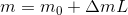
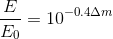
Now we need to understand how light is weakened in the atmosphere, depending on the air mass passed. The law that describes this is called Booger's law
in stellar magnitudes.the law will take a rather simple form:
Where:
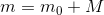
m is the observed magnitude
m0 is the brightness of the star outside the atmosphere
Δm is the atmospheric absorption at the zenith in magnitudes
L is the air mass
Now I’ll talk a little about photometry. When a star’s brightness is measured in a photograph, its magnitude m is given relative to the instrumental magnitude M:
Where m0 is the actual magnitude.
In turn, the instrumental magnitude M will be equal to:
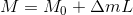
Where M0 is the extra-atmospheric instrumental magnitude.
This is where our absorption hides.
Thus, our main task was to find the absorption at the zenith Δm
Now to practice. First, we need software for photometry. And it will be the workhorse of all astrophotographers - IRIS
The first thing we will do is decode raw.
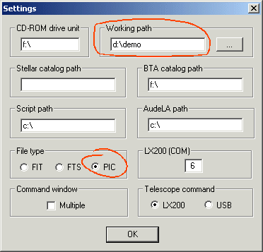
First we set the working directory in File-> Settings.
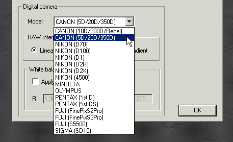
Then we set the camera parameters in Camera settings:
Then finally we decode RAW: Digital photo -> Decode RAW files.
After decoding, press the Done button and the image will appear on the screen. Now we are ready for photometry.
You need to select Analysis-> Aperture photometry. I advise you to simply agree with the drop-down window and get to work. You will have three circles instead of the cursor and your task is to move the center of such a cursor to the star and click. After a click in the Output window, approximately the following data will appear:
We are interested in the last two lines:
Intensity = 52348.0 - intensity in arbitrary units
Magnitude = -11.797 - gloss in instrumental magnitudes (for 0 this brightness is taken whose intensity from one pixel is 1)
Background mean level = 2755.0 - background current in arbitrary units.
Next, you need to open the Stellarium and identify the star. This information should be entered in some table, for example MS Excel.
I did as follows:

In such a table should be entered as much information as possible about the star. Necessarily her catalog gloss (Cat mag), measured gloss (Mag Image) and height, which was determined by the Stellarium (Alt). In order not to get confused, I recommend recording the star number in the catalog (Star name), it is also advisable to record the intensity values and background values.
Then, the atmospheric mass (Airmass) is calculated for each star by height. Then we find the instrumental magnitude Dm as the difference: Dm = Mag image-Cat mag
Please pay attention!It is necessary to enter as much data as possible about stars at different heights, especially at low. After all, the more data, the more accurate the final result. Moreover, we did not take calibration frames and the effects of photometry are affected to varying degrees by noise. On the other hand, Stars are different in color, and as a result, the maximum of their radiation lies at different frequencies, and at different frequencies the absorption can differ significantly ...
Next, you need to build a graph of the dependence of the instrumental magnitude (Dm) on the air mass (Airmass). Select the type of scatter plot. Now, using the least squares method, you need to find the linear equation that is most suitable for this graph. To do this, go to the top menu: Work with diagrams-> Layout-> Trend line-> Additional parameters of the trend line. Here we select the linear type and put a checkmark on the item “Show the equation in the diagram”
. I got a graph like this:
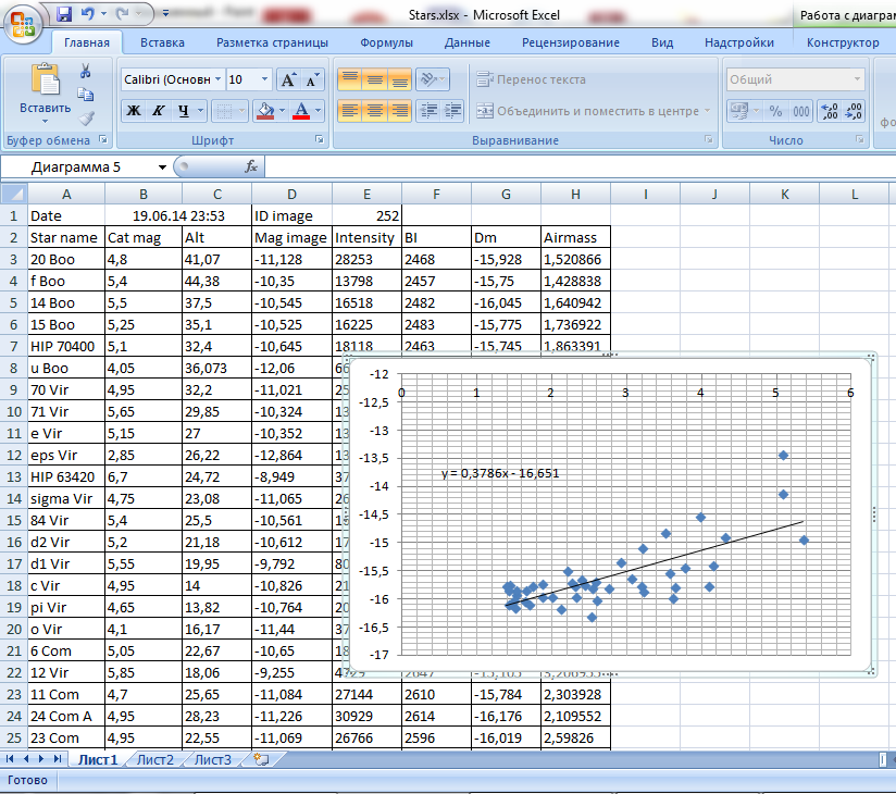
As we see our equation: 0.3786x-16.651.
The coefficient is atmospheric absorption at the zenith and it will be 0.38m, and the free term (-16.7) is an instrumental magnitude without absorption.
Charts in gnuplot:
Dependence on air mass:

Dependence on height:

Strictly speaking, we got a good mark, because The generally accepted average value is 0.44m.
Let us determine how many times the light attenuates the atmosphere according to the Pogson formula:
We obtain that the light is attenuated by 30%. That is, if dust particles are taken from the atmospheric column with a cross section of 1 m2 and placed all of them close to each other, then their area will be 0.3 m2.
It should be noted that the absorption of clean (without impurities) air is 0.2m. Thus, in our city the atmosphere weakens the light by 17% more than clean air ...
We made a fairly simple analysis and did not go into complex processes, such as scattering or the dependence of absorption on the wavelength. However, we got a fairly accurate estimate using just one image. If there is a series of images, then adding them together you can achieve even more accurate results ...
Bit of theory
Our atmosphere is not perfectly transparent: in addition to air there are gas and dust that get there in different ways, in cities, as a rule, due to industrial enterprises or car exhausts. Due to all this, the radiation that passes through the atmosphere is significantly attenuated. And the longer the path that light travels in the atmosphere, the stronger this attenuation. If you look at the figure below, it turns out that the path in the atmosphere is the longer, the lower the height of the light source:
Let's try to derive the dependence of the long path of a light beam in the atmosphere on the height of the light source:
We apply the sine theorem to this triangle:
Using the fact that A = 90 + h, where h is the height of the star, we get:
Further, using the first and last relation from the sine theorem, as well as the theorem on the sum of the angles in a triangle, we get:
Here we used the following:
However, the path length in the atmosphere is usually expressed not in dimension of length, but in dimensionless expressions, i.e. length The paths of a ray of light in the atmosphere are expressed in the heights of a homogeneous atmosphere, and such a unit is called the atmospheric mass (eng: airmass). Let k = R / H be the ratio of the radius of the Earth and the height of a homogeneous atmosphere (k = 800)
Then in the air masses our formula will take the form:
Now we need to understand how light is weakened in the atmosphere, depending on the air mass passed. The law that describes this is called Booger's law
in stellar magnitudes.the law will take a rather simple form:
Where:
m is the observed magnitude
m0 is the brightness of the star outside the atmosphere
Δm is the atmospheric absorption at the zenith in magnitudes
L is the air mass
A little theory about photometry
Now I’ll talk a little about photometry. When a star’s brightness is measured in a photograph, its magnitude m is given relative to the instrumental magnitude M:
Where m0 is the actual magnitude.
In turn, the instrumental magnitude M will be equal to:
Where M0 is the extra-atmospheric instrumental magnitude.
This is where our absorption hides.
Thus, our main task was to find the absorption at the zenith Δm
Practice
Now to practice. First, we need software for photometry. And it will be the workhorse of all astrophotographers - IRIS
The first thing we will do is decode raw.
First we set the working directory in File-> Settings.
Then we set the camera parameters in Camera settings:
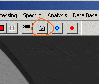
Then finally we decode RAW: Digital photo -> Decode RAW files.
After decoding, press the Done button and the image will appear on the screen. Now we are ready for photometry.
You need to select Analysis-> Aperture photometry. I advise you to simply agree with the drop-down window and get to work. You will have three circles instead of the cursor and your task is to move the center of such a cursor to the star and click. After a click in the Output window, approximately the following data will appear:
Phot mode 3 - (979, 2553)
Pixel number in the inner circle = 197
Pixel number for background evaluation = 816
Intensity = 52348.0 - Magnitude = -11.797
Background mean level = 2755.0
We are interested in the last two lines:
Intensity = 52348.0 - intensity in arbitrary units
Magnitude = -11.797 - gloss in instrumental magnitudes (for 0 this brightness is taken whose intensity from one pixel is 1)
Background mean level = 2755.0 - background current in arbitrary units.
Next, you need to open the Stellarium and identify the star. This information should be entered in some table, for example MS Excel.
I did as follows:
In such a table should be entered as much information as possible about the star. Necessarily her catalog gloss (Cat mag), measured gloss (Mag Image) and height, which was determined by the Stellarium (Alt). In order not to get confused, I recommend recording the star number in the catalog (Star name), it is also advisable to record the intensity values and background values.
Then, the atmospheric mass (Airmass) is calculated for each star by height. Then we find the instrumental magnitude Dm as the difference: Dm = Mag image-Cat mag
Please pay attention!It is necessary to enter as much data as possible about stars at different heights, especially at low. After all, the more data, the more accurate the final result. Moreover, we did not take calibration frames and the effects of photometry are affected to varying degrees by noise. On the other hand, Stars are different in color, and as a result, the maximum of their radiation lies at different frequencies, and at different frequencies the absorption can differ significantly ...
My details
| Date | 06/19/14 23:53 | ID image | 252 | ||||
| Star name | Cat mag | Alt | Mag image | Intensity | BI | Dm | Airmass |
| 20 boo | 4.8 | 41.07 | -11,128 | 28253 | 2468 | -15,928 | 1,520865865 |
| f boo | 5,4 | 44.38 | -10.35 | 13798 | 2457 | -15.75 | 1,428837794 |
| 14 boo | 5.5 | 37.5 | -10,545 | 16518 | 2482 | -16,045 | 1,64094179 |
| 15 boo | 5.25 | 35.1 | -10.525 | 16225 | 2483 | -15,775 | 1,736922288 |
| HIP 70400 | 5.1 | 32,4 | -10.645 | 18118 | 2463 | -15,745 | 1.863391058 |
| u boo | 4.05 | 36,073 | -12.06 | 66655 | 2516 | -16.11 | 1,696331832 |
| 70 vir | 4.95 | 32,2 | -11,021 | 25616 | 2565 | -15,971 | 1,873663569 |
| 71 vir | 5.65 | 29.85 | -10,324 | 13476 | 2556 | -15,974 | 2,005323345 |
| e vir | 5.15 | 27 | -10,352 | 13833 | 2589 | -15,502 | 2.197418439 |
| eps vir | 2.85 | 26.22 | -12,864 | 139837 | 2607 | -15,714 | 2.25757501 |
| HIP 63420 | 6.7 | 24.72 | -8,949 | 3799 | 2614 | -15,649 | 2,384289105 |
| sigma vir | 4.75 | 23.08 | -11,065 | 26671 | 2585 | -15.815 | 2,542206706 |
| 84 vir | 5,4 | 25.5 | -10,561 | 16761 | 2533 | -15,961 | 2,316481972 |
| d2 vir | 5.2 | 21.18 | -10.612 | 17567 | 2631 | -15,812 | 2,756376852 |
| d1 vir | 5.55 | 19.95 | -9,792 | 8067 | 2639 | -15,342 | 2.917077172 |
| c vir | 4.95 | 14 | -10.826 | 21403 | 2656 | -15,776 | 4.092871581 |
| pi vir | 4.65 | 13.82 | -10,764 | 20209 | 2676 | -15,414 | 4,144019169 |
| o vir | 4.1 | 16.17 | -11.44 | 37660 | 2658 | -15.54 | 3,564544399 |
| 6 com | 5.05 | 22.67 | -10.65 | 18196 | 2625 | -15.7 | 2,58533522 |
| 12 vir | 5.85 | 18.06 | -9,255 | 4729 | 2647 | -15.105 | 3,20695548 |
| 11 com | 4.7 | 25.65 | -11,084 | 27144 | 2610 | -15,784 | 2,303928428 |
| 24 Com A | 4.95 | 28.23 | -11,226 | 30929 | 2614 | -16,176 | 2,109551775 |
| 23 com | 4.95 | 22.55 | -11,069 | 26766 | 2596 | -16.019 | 2.598260423 |
| 31 com | 4.9 | 37.07 | -10.961 | 24233 | 2546 | -15,861 | 1,657141284 |
| beta com | 4.2 | 40.93 | -11,658 | 46037 | 2523 | -15,858 | 1,525134451 |
| 37 com | 5.05 | 41.35 | -11,107 | 27728 | 2521 | -16,157 | 1,51242676 |
| HIP 62972 | 6.25 | 42.04 | -9.77 | 8091 | 2500 | -16.02 | 1.492174262 |
| 14 CVn | 5.2 | 45.68 | -10,579 | 17050 | 2481 | -15,779 | 1.396892826 |
| HIP 62641 | 5.85 | 44.53 | -10.011 | 10102 | 2476 | -15,861 | 1.425039994 |
| HIP 64543 | 6.65 | 44.6 | -9,463 | 6099 | 2496 | -16,113 | 1.423277903 |
| HIP 63267 | 7.15 | 24.18 | -8,605 | 2767 | 2613 | -15,755 | 2,43386583 |
| HIP 63221 A | 7.5 | 23,23 | -8,819 | 3371 | 2604 | -16,319 | 2,526815663 |
| delta vir | 3.35 | 18.95 | -12,289 | 82359 | 2620 | -15,639 | 3.063224414 |
| 37 vir | 6 | 18.12 | -9,783 | 8185 | 2620 | -15,783 | 3.19682149 |
| 33 vir | 6.4 | 18,017 | -9,468 | 6129 | 2625 | -15,868 | 3,214259678 |
| HIP 61658 | 5.65 | 15.27 | -9,789 | 8237 | 2643 | -15,439 | 3,765690356 |
| HIP 61637 | 6.3 | 16,4 | -8,518 | 2554 | 2647 | -14.818 | 3,516648775 |
| HIP 60850 | 6.7 | 15.92 | -9.29 | 5201 | 2658 | -15.99 | 3.618160686 |
| eta vir | 3.85 | 10.57 | -11,084 | 27151 | 2690 | -14,934 | 5.357099392 |
| 10 vir | 5.95 | 11.18 | -7,493 | 994 | 2702 | -13,443 | 5,077628047 |
| b vir | 5.35 | 11.18 | -8,788 | 3275 | 2706 | -14,138 | 5,077628047 |
| HIP 58809 | 6.35 | 13.28 | -8,545 | 2618 | 2684 | -14.895 | 4.305596468 |
| 11 vir | 5.7 | 14.42 | -8,837 | 3425 | 2677 | -14,537 | 3.97839932 |
| 17 vir | 6.45 | 15.81 | -9.352 | 5507 | 2657 | -15,802 | 3,642283826 |
Next, you need to build a graph of the dependence of the instrumental magnitude (Dm) on the air mass (Airmass). Select the type of scatter plot. Now, using the least squares method, you need to find the linear equation that is most suitable for this graph. To do this, go to the top menu: Work with diagrams-> Layout-> Trend line-> Additional parameters of the trend line. Here we select the linear type and put a checkmark on the item “Show the equation in the diagram”
. I got a graph like this:
As we see our equation: 0.3786x-16.651.
The coefficient is atmospheric absorption at the zenith and it will be 0.38m, and the free term (-16.7) is an instrumental magnitude without absorption.
Charts in gnuplot:
Dependence on air mass:
Dependence on height:
Strictly speaking, we got a good mark, because The generally accepted average value is 0.44m.
What does this give us?
Let us determine how many times the light attenuates the atmosphere according to the Pogson formula:
We obtain that the light is attenuated by 30%. That is, if dust particles are taken from the atmospheric column with a cross section of 1 m2 and placed all of them close to each other, then their area will be 0.3 m2.
It should be noted that the absorption of clean (without impurities) air is 0.2m. Thus, in our city the atmosphere weakens the light by 17% more than clean air ...
Conclusion
We made a fairly simple analysis and did not go into complex processes, such as scattering or the dependence of absorption on the wavelength. However, we got a fairly accurate estimate using just one image. If there is a series of images, then adding them together you can achieve even more accurate results ...