grep July 18, 2014 at 00:29

Experiments with bit-reversed patterns in two-dimensional additive cellular automata

Somehow I experimented with cellular automata. With one-dimensional and two-dimensional. I thought up on what initial state to apply some rule. When, as the initial state of a two-dimensional cellular automaton, I began to use a bit-reversal permutation of the diagonal line, then after using the automaton we got peculiar patterns. From time to time, distinctive characteristic patterns appeared among the patterns. I highlighted these patterns and experimented with them a bit. With what I managed to find out, I share in this article.

In the article I will briefly talk about additive cellular automata. I will also give a sequence of my observations and tasks that I set. Each stage will be accompanied by images of the state of the cellular automaton. In addition, for better visualization, I wrote a web application that will add interactivity when reading an article. The application is based on React and should work in modern browsers. I will also accompany some actions with links to pieces of code in Python.

Disclaimer: The article is purely informative and entertaining in nature, since I am not aware of the applications of the proposed information. Also, I’m interested in sorting out the fragmentary information that I managed to find out. And, perhaps, to find roughness in them. Perhaps new experiments will come to my mind.

I hope that the article will entertain you, although I will write clearly and on the case.

Preliminary acquaintance with cellular automata

If you are not familiar with cellular automata (CA) or just heard about them, then I suggest that you read the introductory articles:

Toffoli T., Margolus N., Overview of cellular automata ( pdf ) on The Game of Life by Roman Parpalak - a good introduction to CA.

Evgeny Zolotov, Boxed World ( pdf ) at Computra.

More practical articles:

OCo, Cellular Automata ( pdf ) on Programs, Fractals and Sundries from OCo - a brief introduction to cellular automata and examples of the implementation of various cellular automata.

Matvey Kotov ( mkot ), A little about cellular automata on Habré.

Tatyana Bibikova, Hydrodynamics of the sea urchin sperm ( pdf ) - a story about scientific work.

I will also give some interesting materials, in my opinion, in English:

Elementary Cellular Automaton at WolframMathWorld - an approach to enumerating CA rules is described and illustrations of the behavior of all the rules for a certain starting state are given.

Elementary cellular automaton on Wikipedia - about the same as the previous one. But there are illustrations of the application of certain rules in a random starting state.
Rafael Espericueta, Cellular Automata Dynamics ( pdf ) - an illustrated book about zero-dimensional, one-dimensional and two-dimensional spacecraft.
Additive Cellular Automatonat WolframMathWorld - about additive spacecraft.

Mirek Wojtowicz, 1D and 2D Cellular Automata explorer - the site has a collection of CA rules.

Two-dimensional additive cellular automaton

A cellular automaton has a state and a rule by which a transition from the previous state to the next occurs.

The state of a two-dimensional CA is a two-dimensional array of cells. In our case, this array has the same length and width N. Each cell can take values 0 or 1. We will represent cells with a value of 0 in black, and cells with a value of 1 in white.

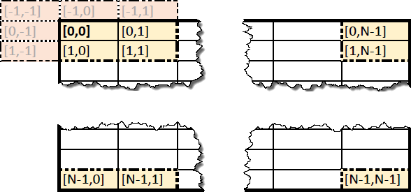
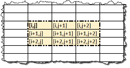
The position of the cell in the spacecraft's state array is described by the coordinates [i, j], where i, j take values from 0 to N-1, moreover, i is the column number, and j is the row number.

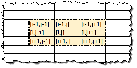
A rule is a procedure that calculates the value of a cell for the next state based on the value of the cell and the value of the neighboring eight cells. The set of cells that can participate in the calculation of the rule will be called a neighborhood. This is what the cell neighborhood [i, j] looks like:

The procedure for calculating the rule is applied in parallel and the same for all cells of the CA state for which all neighboring cells are defined (in a typical implementation, sequentially using two state arrays.) A single application of the rule to all cells will be called one iteration.

At the boundaries of the CA state, not all neighboring cells are defined. There are various ways to identify missing cells. And each method gives a different result. In our case, the missing neighboring cells will be taken from opposite edges of the state. Thus, our array, as it were, is “glued” to the left edge with the right, and the upper edge with the lower. Such a “gluing” emulates the surface of a torus, or it is also called a toroidal lattice.

.
Perhaps the most famous example of a two-dimensional spacecraft is the game "Life" .

For a two-dimensional additive cellular automaton (AKA), the rule calculation procedure calculates the sum modulo 2(same as XOR) values of certain cells from nine cells from the vicinity of the calculated cell. In our case, the value of the cell is included in the sum no more than once.

We denote the calculated cell with coordinates [i, j] as c ₁ , and the neighboring cells as c ₂ , c ₄ , c ₈ , c ₁₆ , c ₃₂ , c ₆₄ , c ₁₂₈ and c ₂₅₆ with the location according to the diagram:

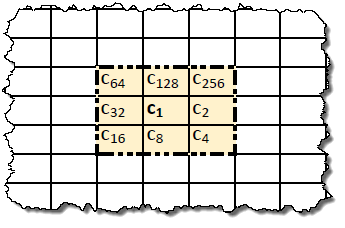
As you noticed, neighborhood cell indices take values of the form 2 ⁿ, where n varies from 1 to 9. Such indices are very convenient, since the sum of arbitrary indices gives a number that uniquely determines in binary representation which cells are included in the sum for calculating the rule. This number will be the rule number.

For example, rule 15 . According to the binary representation 15 = 000001111 ₂ , it decomposes into terms 000000001 ₂ , 000000010 ₂ , 000000100 ₂ , 000001000 ₂ or 1, 2, 4 and 8. Hence, rule 15 means that each cell of a new state is the sum of cells from ₁ , s ₂ , s ₄ and s ₈previous state. Other neighboring cells do not participate in the calculation of the rule. Thus, the rule calculation procedure will be an expression with ₁ [t] = c ₁ [t-1] + c ₂ [t-1] + c ₄ [t-1] + c ₈ [t-1] (mod 2), where c ₁ [t] is the cell of the new state, and c ₁ [t-1], c ₂ [t-1], c ₄ [t-1], c ₈ [t-1] are the cells of the previous state, and the coordinates cells with ₁ [t] and ₁ [t-1] coincides, and cells with ₂ [t-1], ₄ [t-1], ₈ [t-1] are adjacent cells of the cell with ₁[t-1] according to the diagram.

The idea of such a numbering of AKA rules is taken from [ Khan1997 ].

In the application, you can interactively set the rule, both by number and by checking the boxes with cells in the neighborhood. When you change one view, another view will change automatically.

The entire article is based on the use of rule 15. There will also be a couple of experiments using rule 511 .

Preliminary identification of the manifestation of the permutation of the diagonal line

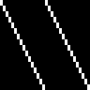
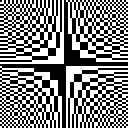
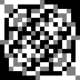
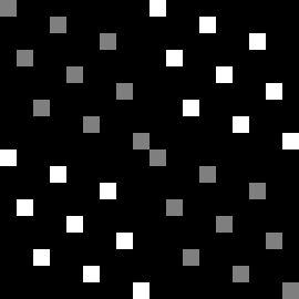
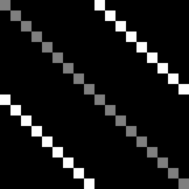
Take the empty state AKA 64x64 cells, and draw a diagonal line :

.
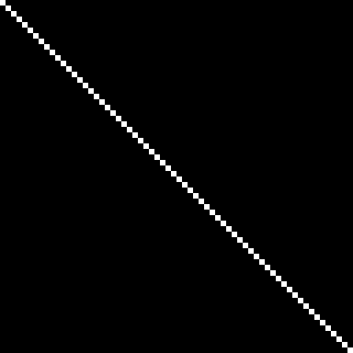Apply bit-reversed permutation of lines. Or columns. No difference. What is bit reversal and bit reversal permutation I have already written. [ BRH2012 ] In the application, this is done using the BRP (y) button or by selecting the “Permuted Diagonal Line” Pattern. We obtain state :

.

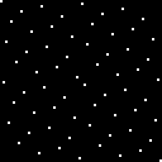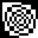
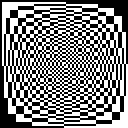
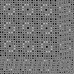
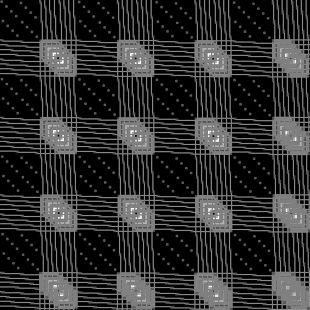
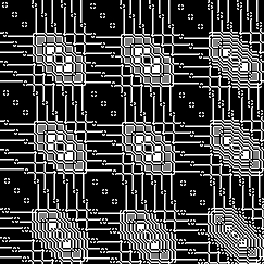
Now we iteratively apply to this rule of 15 ( «Apply rule» button.) After 30 iterations, we obtain the condition:

.
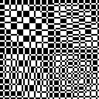My eye is already set, and I can easily recognize the patterns I are looking for. From this state, one can distinguish something that has an 8x8 size consisting of virtual black and white cells, repeated four times with different drawing methods. Highlight this explicitly:

.
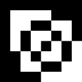It would seem some kind of set of cells. Indeed, each iteration gives a certain pattern. Why did I highlight this iteration and this drawing?

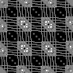
Let's take an AKA 128x128 cell . And we will do the same. Let us consider the iteration 62. We see the condition:

Experiment without comment

Press the BRP (x, y) and 4BRP (x, y) permutation buttons in a different sequence. Similar permutations can be achieved with the PG (x, y) button. Thus, you can get the pattern in its pure form without recognition of virtual cells.

We see virtual cells that specify a 16x16 pattern. Isolate him

.

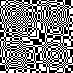
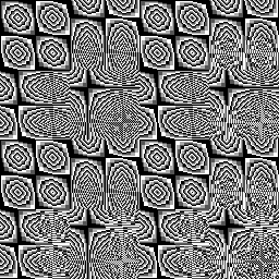
To be sure, take AKA 256x256 cells . That is the state in the iteration 60:

.
We see virtual cells defining the familiar 8x8 cell pattern. The only difference is the way the virtual cells are drawn. At the following iterations, the pattern is repeated in a particular rendering method. For example, 62 iterate:

.
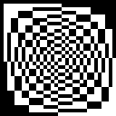
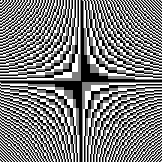
Finally, 126 iteration:

.
Recognizable picture, is not it? Also, pay attention to the dynamic moire with the smooth movement of this pattern on your LCD monitor. But this is a topic for another article. Select from the virtual cell pattern 32x32:

.

This was enough for me to be seized by interest in this object and to explore it more deeply. We call this object a manifestation of a permutation of the diagonal line or PPDL.

I decided to figure out how to generate such patterns in their pure form without doing many iterations of the AKA and not recognizing virtual cells.

Generation of the manifestation of a diagonal line permutation

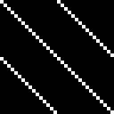
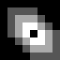
Take the PPDL in its purest 32x32 cells . Apply the Rule 15 (from the beginning I experimented only with rule 225 , which led to the emergence of unnecessary amendments in generating PPDL.) Get the state:

.
If we tinker a bit with this state, we can come to the conclusion that in each quarter a bit-reversal permutation of the diagonal line is depicted. Check this by pressing the 4BRP (y) button. We get

.
Also, you can not rearrange each quarter separately, but rearrange the entire status bar . Then we get two diagonal lines. It would seem that it makes no difference which approach to choose. But, when moving to an arbitrary module / base, with the first option, the generation is simpler. (From the very beginning, in my experiments, I used the second method. And I finally came to the first method right when I wrote the article.)

And so, we know the state of the AKA after applying rule 15. And this state is easy to generate for a given size.

It remains to reverse this state. Let us write down rule 15 again:
with ₁ [t] = s ₁ [t-1] + s ₂ [t-1] + s ₄ [t-1] + s ₈ [t-1] (mod 2), where s ₁[t] is a known state cell containing permutations of diagonal lines in each quarter, and with ₁ [t-1], with ₂ [t-1], c ₄ [t-1], and ₈ [t-1] are unknown PPDL cells. If you look at the detected PDLs of various sizes, it is easy to notice that the cells of the first row and first column contain only zeros. Thus, we assume that we already know the significance of the first PPDL cells. Based on these values, it becomes possible to find the remaining values of the PPDL cells.

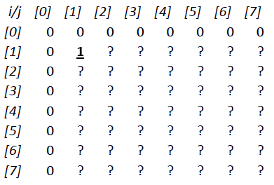
For example, take an AKA of 8x8 cells. The state t with permutations of diagonal lines in each quarter is depicted in the form of a table:

Let us depict in the form of a table the desired state of the PDL t-1 with the known first row and first column:

Three known cells in the upper left corner will correspond to the terms of rule 15: with ₁ [t-1], with ₂ [t-1], with ₈ [t-1]. An unknown cell [1,1] corresponds to the term with ₄ [t-1]

.

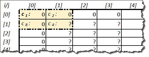Other terms in rule 15 are not involved.

We solve the equation for c ₄ [t-1]. We get:
s ₄ [t-1] = s ₁ [t] + s ₁ [t-1] + s ₂ [t-1] + s ₈ [t-1] (mod 2) (when modulo 2 is added, the sign minus does not matter.) According to the tables, with ₄ [t-1] = 1 + 0 + 0 + 0 = 1 (mod 2). We get the state:

Similarly, the calculated cell [1, 2] or cell [2, 1] with the offset:

.
Etc. Cell by cell, line by line , we get the state:

* * *

Also, PPDL can be generated using block-recursive construction of matrices . If this is interesting to someone, then you can try to do it yourself.

Some properties of the manifestation of the permutation of the diagonal line

Property 1

PPDL has size N equal to the power of two, i.e. N = 2 ⁿ .

Property 2

The cells of the first row and first column are zero.

Property 3

Even cells on row N / 2 and column N / 2 are equal to one, and odd cells are equal to zero. In other words, they are equal to the corresponding cell coordinate taken modulo 2.

Property 4

If we apply rule 15 to the PDL, then we get a state that contains permutations of the diagonal line in each quarter.

Property 5

Prepare PPDL 64x64 cells :

.
And we will apply the rule 511. In iteration 16, we get:

.
This is the same pattern, only shifted 32 cells diagonally.

A similar pattern occurs with PPDL of other sizes.

The pattern obtained in this way can be generated in the same way as the main one, only you need to take the first row and first column, which consist of units on even cells .

It should be noted that this is not a unique property of this pattern. You can come up with other states of the AKA that have the same property.

If we continue to apply rules 511, then at iteration 32, the original image will return. The original image is restored with any combination of AKA state cells, but not with any state size. This property of rule 511 is proposed for use in cryptography. [ Chatz2012 ] From this source, I learned about the ability to use rule 511 in my experiments.

* * *

Exploring other areas, I came across the fact that if there are objects in which calculations with module 2 are applied, then they can be expanded to an arbitrary module> = 2.

Manifestation of permutation of a diagonal line with an arbitrary module / base

First, we expand the rule calculation procedure. Now, computing the rule will calculate the sum of the selected neighborhood cells taken modulo M> = 2. That is, after we calculate the sum of the values of the selected cells, we will take the remainder of the division by the number M as the final value of the cell. Thanks to the calculation modulo M, the cells of the AKA state will take integer values from 0 to M-1.

We will depict cells with a value of 0 in black, cells with an M-1 value will be depicted in white, and intermediate values of cells will be depicted in intermediate shades of gray.

Something about an AKA with a module> = 2 is in [ CAD1997 ].

Also, you need to go from the reverse bit, which is the reverse of the digits with the base 2, toreverse of digits with an arbitrary base B> = 2. Digit reversal will allow a digital-reverse permutation of the diagonal line (I'm not quite sure I entered the terms correctly. I thought about the options: digit / digit reversal and digit-reversal permutation. But, in my opinion, this looks awful.) It will also be incorrect if the size of the state of the AKA will be a power of 2. You need to adjust the size of the state of the AKA. Now this size N will be some degree of base B, i.e. will have the form N = B ⁿ .

We’ll experiment with rule 15. The module and base must match. Time . Two .
In the second case, 62 iterate manifested something remotely similar:

.
There are virtual cells, but all this is not that.

Stumbled in while writing an article ...

At iteration 125, the following state appears:

If we apply the permutation PG (x, y) three times, we get fragments with the desired pattern:

Then I tried rule 511 . Take the permutation of a diagonal line with module / base 3 and size 243x243. At iteration 26 obtain

.
Clearly visible virtual cell 5x5 (more correctly 6x6), and a recognizable pattern:

.
Take the permutation of a diagonal line with module / base 3 and size 729x729 . At iteration 80, we get a 18x18 virtual pattern .

Similar results can be obtained if you take a permutation of the diagonal line with module / base 4. But for this you will have to calculate a rule with a neighborhood of 4x4 , which is not implemented in the application. I can only show the finished results. At iteration 42 we get 8x8 virtual pattern .

Let's try to find a way to generate PDLs as we did before.

Take PPDL 18x18 cell module / base 3:

.
We apply rule 15 and get a terrible mess:

.
Start over. Apply rule 511 :

.
Already better. But still a lot of superfluous. And it’s not a desire to reverse the state according to rule 511.

After a while, it occurred to me to experiment with signs of the terms of the AKA rule. To indicate which terms are used with a minus sign, I suggest writing another number after the rule number, which uses the same encoding as the rule.

For example, rule 15-10. It includes the terms c ₁ , c ₂ , c ₄ , c ₈ . But the terms c ₂ and c ₈ enter with a minus sign. We get the function c ₁ [t] = c ₁ [t-1] -c ₂ [t-1] + c ₄ [t-1] -c ₈ [t-1] (mod M)

Rule 15-5 gives the state:

.
A typically 15-10 gives the state:

.
Let us dwell on rule 15-10. Since the cells in the upper left quarter contain units (gray cells.) Whereas after rule 15-5, there are deuces (white cells.) And the unit is closer to the beginning of the numerical axis.

Apply the digital-to reverse a permutation of rows in each quarter of the last state button 4DRP (y) and obtain

.
The state can be divided into quarters, and in each of them a diagonal line with the corresponding value.

And so, we became aware of the condition that needs to be obtained after applying rule 15-10. It remains to reverse this state. We write the rule 15-10:
c ₁ [t] = c ₁ [t-1] -c ₂ [t-1] + c ₄ [t-1] -c ₈ [t-1] (mod M), where c ₁ [t] is a known state cell containing permutations of diagonal lines in each quarter with the corresponding value, and with ₁ [t-1], with ₂ [t-1], c₄ [t-1], s ₈ [t-1] - unknown PPDL cells, M - module (currently it is 3.). Fix values with ₁ [t-1], s ₂ [t-1], s ₈ [t-1] as we did before. We solve the equation for c ₄ [t-1]. We get:
c ₄ [t-1] = c ₁ [t] -c ₁ [t-1] + c ₂ [t-1] + c ₈ [t-1] (mod M). After calculating all the unknown cells, we get the desired pattern.

Thus, obtaining patterns with a module / base M> = 2 is similar. We need to take a state, a quarter of which has a size, in the form of the degree of foundation. In each quarter, draw diagonal lines with a digitally reversible permutation. The cells in the upper left and lower right quarters take the value 1. And the other two quarters take the value M-1. Then reverse the resulting state according to rule 15-10. Source code .

The only thing that confuses is that the pattern was identified using rule 511-0. To make sure that the guesswork is correct, we will check rule 15-10 on the rearranged diagonal line . At iteration 52 obtain

.
The picture is identical to that obtained previously using rule 511-0 up to an offset.

This bias would not be ...

Если немного изменить способ вычисления правила 511. Сейчас мы вычисляем правило 511 в окрестности с основной клеткой по центру. А в правиле 15-10, с учетом только задействованных клеток, основная клетка лежит в углу. Мы можем устранить эту разницу, изменив вид окрестности для правила 511 таким образом:

Вот куски кода, которые реализуют описанные варианты:

Experiments with other dimensions of the AKA state using rule 15-10 give patterns with virtual cells that match the PDL that is generated by the above algorithm.

* * *

I also managed to implement the generation of PDL with the base / module 3 using block-recursive matrix construction. Examining the block structure of PPDL, I noticed that the structure of blocks becomes more and more complicated with an increase in module / base. An element similar to the matrix of the discrete Fourier transform (that is, a matrix in the form of a multiplication table modulo.) Also becomes noticeable. But I do not want to overload this article with a detailed study in this direction. Maybe someone will be more interested in studying this on their own.

* * *
Let us revise the properties of PPDL.