Optimization of the geometric algorithm for training ANNs in the analysis of independent components
Good afternoon, dear Khabrovites. Perhaps many of you will be wondering: “Where is the description of the main algorithm?”
So, links to sources will be indicated below, and I will not rewrite the main algorithm.
I’ll explain right away. This article is the result of my research work, and later on the topic of my diploma.
But enough introductory words. Go!
ANNs are an attempt to use the processes occurring in the nervous systems of living things to create new information technologies.
The main element of the nervous system is a nerve cell, abbreviated as a neuron. Like any other cell, the neuron has a body called the catfish, inside which the nucleus is located, and numerous processes come out - thin, densely branching dendrites, and a thicker axon splitting at the end (Fig. 1).

Fig. 1. Simplified structure of a biological nerve cell.
Input signals enter the cell through synapses, the output signal is transmitted by the axon through its nerve endings (collaterals) to the synapses of other neurons, which can be located either on dendrites or directly on the cell body.
Let us consider it as the main used model of multilayer NS of direct distribution. A multilayer network consists of neurons located at different levels, when, in addition to the input and output layers, there is at least one intermediate (hidden) layer. The generalized structure of a two-layer NS is shown in (Fig. 2).

Fig. 2. The generalized structure of a two-layer NS (with one hidden layer)
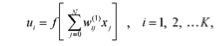
The output signal of the i-th neuron of the hidden layer can be written as
output signals
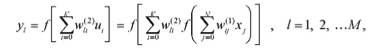
To isolate the signals of sources S (t) contained in the signal mixture, we use the adaptive filter structure based on a single-layer ANN (Fig. 3), proposed in the 80s by Herolt and Jutten, where X is the matrix of vectors of the observed signals formed in accordance with the equation ( 1) using an unknown mixing matrix A, W is the matrix of weights of the neural network.
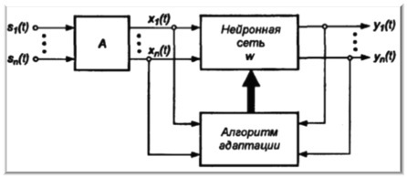
Fig. 3. The block diagram of the adaptive filter on the ANN
So, as you know, any neural network requires training.
There are various learning algorithms, with a teacher, without a teacher, combined.
In this paper, we considered a rather unusual algorithm for training ANNs - geometric.
To begin, consider its main differences:
The following situation was investigated in the work.
A mixture of various signals arrives at the input (I emphasize in advance that the number of signals is already known).
It was necessary to develop such an algorithm for training a neural network that would allow to separate signals from a mixture with maximum accuracy.
Figure 4a shows the source signals. It is noticeable that 2 independent components are clearly distinguished, each of which describes the signal.
Figure 4b shows a mixture of signals. The signals correlate with each other, and it becomes quite difficult to distinguish between them (try superimposing one image on another).

Fig. 4. Geometric interpretation of multiplication by a matrix A
(a) - signals of sources, b) - signals of mixtures)
From (1) it is clear that a mixture of signals obtained by multiplying the source signals in the mixing matrix A:
 ,
,
which is in turn represented as a rotation matrix:
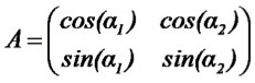 .
.
From this rather simple idea, the geometric algorithm for training ANNs was born - histGEO.
The task of the reconstruction stage of the mixing matrix is to find the
angles α1 and α2 of the rotation matrix. In the general case, the number of angles is equal to the number of independent components
involved in mixing.
Briefly, the functioning of histGEO for processing
super - Gaussian signals can be described as follows:
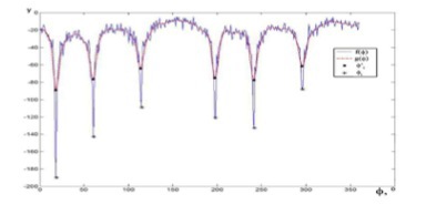
Fig. 5. Search for angles φ i using gradient descent.
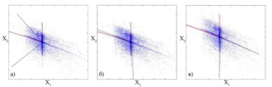
Fig. 6.1. Evaluation results of the mixing matrix for 2 audio signals
(a - geoica, b-fastgeo, c - histgeo)
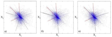
Fig. 6.2. Evaluation results of the mixing matrix for 3 audio signals.
The case of a crowded basis
(a - geoica, b - fastgeo, c - histgeo)
Practical studies of the work of the considered algorithms were carried out in the
mathematical modeling system Matlab 7.5 using the extension packages
fastICA, geoICA, ICALab (extensions for training. The
work was divided into two parts with increasing complexity of separation:

Fig. 7.1. Characteristics of the source signals: the form of the source signals
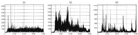
Fig. 7.2. Characteristics of the initial signals: frequency spectra
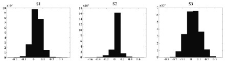
Fig. 7.3. Characteristics of the initial signals: probability distributions
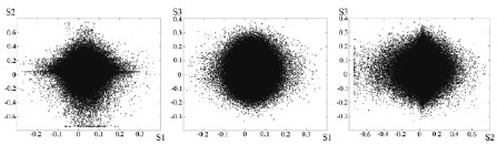
Fig. 7.4. Characteristics of the original signals: scatter plots
In addition to the frequently encountered super-Gaussian distribution (audio signals, images, video signal, etc.),
there are so-called sub-Gaussian signals (various kinds of noise, statistical values, competition of individuals of the same species in nature).
And it is sometimes unimaginably difficult to separate signals of this type, because they are presented in an implicit form and greatly complicate the distribution pattern.
Oddly enough, fairly simple geometric algorithms were able to solve this problem.
It is enough to choose the right geometrical characteristic characterizing the independent component.
The signals at the ANN outputs will have the form
i.e. the linear filtering problem is reduced to finding the correct values of the coefficients of the
matrix of weights of the neural network W.
From a comparison of the scattering diagrams of the initial sources and the obtained mixtures X
(Fig. 8), it can be concluded that multiplication by the mixing matrix A is equivalent to the
rotation of the independent components by some angles α1 and α2 in the x1Ox2 plane.
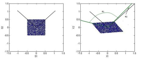
Fig. 8. Geometric interpretation of multiplication by the mixing matrix A
(a - source signals, b - mixture signals)
To convert the data into a convenient form for work, it was necessary
to carry out the decorrelation procedure for a set of signals (“bleaching”),
which converts their joint correlation matrix into a
diagonal shape, by elements which are the variances of these
signals (Fig. 9). And the diagonal of the square turned out to be the desired geometric feature:
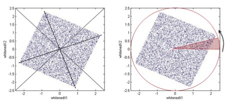
Fig. 9. Decorated (“bleached”) signals X1 and X2.
(a - search for a suitable geometric feature, b - construction of a distribution histogram)
From the conditions for the points to enter the circle sector - obviously larger
in area than the area of the analyzed distribution (Fig. 9b) - the
density distribution of points in the sector was calculated as a
function of angle φ ( fig.
10 ): fig. 10. The search for the angles φ i in the histgeo algorithm
where f * (φ) - f (φ), “smoothed” using a filter.
To reduce the error has been generated array of values of deviation relative to the starting 4 diagonals diagonals respectively (45 a , 135 a , 225 a , 315o ) (Fig. 11), then the average value of the deviations was found.
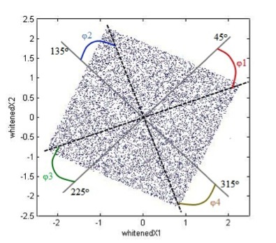
Fig. 11. Search for the angles of deviation of the diagonals from the given angles.
Knowing the angle at which the diagonals are rotated, as well as the fact that the diagonals intersect in the center of the square, you can rotate all points relative to this center by this angle towards the corresponding diagonals. To do this, it is necessary to calculate the recovery matrix:
The resulting distribution graphically coincides with the initial one, which is
clearly shown in Fig
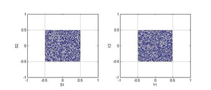
. 12: Fig . 12 . Comparison of the reference distribution of S (a) and reduced Y (b).
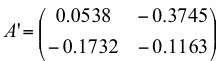
To find the mixing matrix A ', it is necessary to use the
procedure inverse to the decorrelation procedure. The resulting matrix
has the form:
Mutual influence error between matrices A and A ':
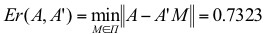
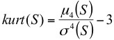
Table 1. Kurtosis coefficients for matrices S, X, Y:
Kurtosis ratio:
At this stage, it cannot be said that the algorithm is universal and applicable in the case of non-square mixing matrices for any class of distributions, but it can be noted with confidence that in the case of square matrices this algorithm copes with its task.
List of references:
So, links to sources will be indicated below, and I will not rewrite the main algorithm.
I’ll explain right away. This article is the result of my research work, and later on the topic of my diploma.
But enough introductory words. Go!
1. Artificial neural networks
ANNs are an attempt to use the processes occurring in the nervous systems of living things to create new information technologies.
The main element of the nervous system is a nerve cell, abbreviated as a neuron. Like any other cell, the neuron has a body called the catfish, inside which the nucleus is located, and numerous processes come out - thin, densely branching dendrites, and a thicker axon splitting at the end (Fig. 1).
Fig. 1. Simplified structure of a biological nerve cell.
Input signals enter the cell through synapses, the output signal is transmitted by the axon through its nerve endings (collaterals) to the synapses of other neurons, which can be located either on dendrites or directly on the cell body.
2. Multilayer perceptron
Let us consider it as the main used model of multilayer NS of direct distribution. A multilayer network consists of neurons located at different levels, when, in addition to the input and output layers, there is at least one intermediate (hidden) layer. The generalized structure of a two-layer NS is shown in (Fig. 2).
Fig. 2. The generalized structure of a two-layer NS (with one hidden layer)
The output signal of the i-th neuron of the hidden layer can be written as
output signals
To isolate the signals of sources S (t) contained in the signal mixture, we use the adaptive filter structure based on a single-layer ANN (Fig. 3), proposed in the 80s by Herolt and Jutten, where X is the matrix of vectors of the observed signals formed in accordance with the equation ( 1) using an unknown mixing matrix A, W is the matrix of weights of the neural network.
X = AS (1)Fig. 3. The block diagram of the adaptive filter on the ANN
3. The use of geometric algorithms for training ANN
So, as you know, any neural network requires training.
There are various learning algorithms, with a teacher, without a teacher, combined.
In this paper, we considered a rather unusual algorithm for training ANNs - geometric.
To begin, consider its main differences:
- Intuitive and clear
- High speed data processing
- Possibility of using for non-square mixing matrices (only in the case of super-Gaussian distributions)
- Easy to program
The following situation was investigated in the work.
A mixture of various signals arrives at the input (I emphasize in advance that the number of signals is already known).
It was necessary to develop such an algorithm for training a neural network that would allow to separate signals from a mixture with maximum accuracy.
Figure 4a shows the source signals. It is noticeable that 2 independent components are clearly distinguished, each of which describes the signal.
Figure 4b shows a mixture of signals. The signals correlate with each other, and it becomes quite difficult to distinguish between them (try superimposing one image on another).
Fig. 4. Geometric interpretation of multiplication by a matrix A
(a) - signals of sources, b) - signals of mixtures)
From (1) it is clear that a mixture of signals obtained by multiplying the source signals in the mixing matrix A:
, which is in turn represented as a rotation matrix:
. From this rather simple idea, the geometric algorithm for training ANNs was born - histGEO.
4. The histGEO algorithm for the case of super-Gaussian distributions.
The task of the reconstruction stage of the mixing matrix is to find the
angles α1 and α2 of the rotation matrix. In the general case, the number of angles is equal to the number of independent components
involved in mixing.
Briefly, the functioning of histGEO for processing
super - Gaussian signals can be described as follows:
- the scattering diagram of the components of the matrix X is constructed;
- the probability density distribution is calculated as a function of the angle φ: f = f (φ);
- the resulting distribution is processed using an averaging software filter to smooth the surface of the obtained function, while maintaining the location of the extrema;
- roughly determine the places of possible localization of the minima of the function g = -f (φ), where f (φ) is the “smoothed” g (φ));
- using the gradient descent algorithm, the coordinates of the angles φ i are refined (Fig. 5.)
Fig. 5. Search for angles φ i using gradient descent.
- the coefficients of the reducing matrix are calculated M
where n is the number of independent components in the mixture; - at the stage of testing the algorithm, the obtained values of the angles φ; plotted on the scattering diagram and compared with α (Fig. 6.1-6.2)
Fig. 6.1. Evaluation results of the mixing matrix for 2 audio signals
(a - geoica, b-fastgeo, c - histgeo)
Fig. 6.2. Evaluation results of the mixing matrix for 3 audio signals.
The case of a crowded basis
(a - geoica, b - fastgeo, c - histgeo)
Audio processing
Practical studies of the work of the considered algorithms were carried out in the
mathematical modeling system Matlab 7.5 using the extension packages
fastICA, geoICA, ICALab (extensions for training. The
work was divided into two parts with increasing complexity of separation:
- Evaluation of the mixing matrix in a square matrix problem, the signals of S sources - speech, noise, music (Fig. 7.1-7.4)
- Estimation of the mixing matrix in a problem with a crowded basis, S source signals - speech, noise, music
Fig. 7.1. Characteristics of the source signals: the form of the source signals
Fig. 7.2. Characteristics of the initial signals: frequency spectra
Fig. 7.3. Characteristics of the initial signals: probability distributions
Fig. 7.4. Characteristics of the original signals: scatter plots
5. The histGEO algorithm for the case of sub-Gaussian distributions.
In addition to the frequently encountered super-Gaussian distribution (audio signals, images, video signal, etc.),
there are so-called sub-Gaussian signals (various kinds of noise, statistical values, competition of individuals of the same species in nature).
And it is sometimes unimaginably difficult to separate signals of this type, because they are presented in an implicit form and greatly complicate the distribution pattern.
Oddly enough, fairly simple geometric algorithms were able to solve this problem.
It is enough to choose the right geometrical characteristic characterizing the independent component.
The signals at the ANN outputs will have the form
Y=WX (2)i.e. the linear filtering problem is reduced to finding the correct values of the coefficients of the
matrix of weights of the neural network W.
From a comparison of the scattering diagrams of the initial sources and the obtained mixtures X
(Fig. 8), it can be concluded that multiplication by the mixing matrix A is equivalent to the
rotation of the independent components by some angles α1 and α2 in the x1Ox2 plane.
Fig. 8. Geometric interpretation of multiplication by the mixing matrix A
(a - source signals, b - mixture signals)
To convert the data into a convenient form for work, it was necessary
to carry out the decorrelation procedure for a set of signals (“bleaching”),
which converts their joint correlation matrix into a
diagonal shape, by elements which are the variances of these
signals (Fig. 9). And the diagonal of the square turned out to be the desired geometric feature:
Fig. 9. Decorated (“bleached”) signals X1 and X2.
(a - search for a suitable geometric feature, b - construction of a distribution histogram)
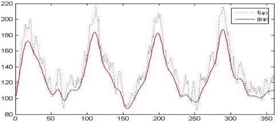
From the conditions for the points to enter the circle sector - obviously larger
in area than the area of the analyzed distribution (Fig. 9b) - the
density distribution of points in the sector was calculated as a
function of angle φ ( fig.
10 ): fig. 10. The search for the angles φ i in the histgeo algorithm
f=f(φ)g(φ)=f*(φ) , where f * (φ) - f (φ), “smoothed” using a filter.
To reduce the error has been generated array of values of deviation relative to the starting 4 diagonals diagonals respectively (45 a , 135 a , 225 a , 315o ) (Fig. 11), then the average value of the deviations was found.
Fig. 11. Search for the angles of deviation of the diagonals from the given angles.
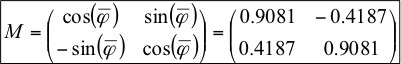
Knowing the angle at which the diagonals are rotated, as well as the fact that the diagonals intersect in the center of the square, you can rotate all points relative to this center by this angle towards the corresponding diagonals. To do this, it is necessary to calculate the recovery matrix:
The resulting distribution graphically coincides with the initial one, which is
clearly shown in Fig
. 12: Fig . 12 . Comparison of the reference distribution of S (a) and reduced Y (b).
To find the mixing matrix A ', it is necessary to use the
procedure inverse to the decorrelation procedure. The resulting matrix
has the form:
Mutual influence error between matrices A and A ':
Table 1. Kurtosis coefficients for matrices S, X, Y:
| S | X | Y | |
| kurt1 | -0.8365 | -0.7582 | -0.8379 |
| kurt2 | -0.8429 | -0.8341 | -0.8465 |
Kurtosis ratio:
6. Conclusions
- The possibility of applying the histGEO geometric algorithm to the class of sub-Gaussian distributions is tested.
- Despite the apparent simplicity, geometric algorithms represent an effective mechanism for training ANNs in adaptive filtering problems.
- The developed optimized version of the histGEO algorithm is applicable to both super-Gaussian and sub-Gaussian type signals.
- With an increase in the number of sources included in the mixture, it becomes more difficult to make the correct matrix estimation, since the extrema of the function g (φ) become less pronounced and it is possible that the solution falls into one of the local minima.
- The effectiveness of the algorithm in the case of separation of signals with an overcrowded basis (variants of a non-square mixing matrix) requires additional research.
At this stage, it cannot be said that the algorithm is universal and applicable in the case of non-square mixing matrices for any class of distributions, but it can be noted with confidence that in the case of square matrices this algorithm copes with its task.
List of references:
- Khaikin S. Neural networks: full course / S. Khaikin. - M.: Williams Publishing House, 2006. - 1104 p.
- Bormontov E.N., Klyukin V.I., Tyurikov D.A. Geometric Learning Algorithms in the Problem of Analysis of Independent Components / E. N. Bormontov, V. I. Klyukin, D. A. Tyurikov - Vestnik VGTU, t.6, No. 7. - Voronezh: VSTU, 2010.
- A. Jung, FJ Theis, CG Puntonet EW Lang. Fastgeo - a histogram based approach to linear geometric ICA. Proc. of ICA 2001, pp. 418-423, 2001.
- FJ Theis. A geometric algorithm for overcomplete linear ICA. B. Ganslmeier, J. Keller, KF Renk, Workshop Report I. of the Graduiertenkolleg, pages 67-76, Windberg, Germany, 2001.
- G.F. Malykhina, A.V. Merkusheva Robust methods for separating a mixture of signals and analysis of independent components with noisy data / G.F. Malykhina, A.V. Merkusheva SCIENTIFIC INSTRUMENT, 2011, volume 21, No. 1, p. 114–127
- XIX International Scientific and Technical Conference "Radar, Navigation, Communication" (RLNC-2013) Section 1. Optimization of the geometric algorithm for training ANNs in the analysis of independent components. E.N. Bormontov, V.I. Klyukin, D.A. Tyurikov - 2013