λ-calculus. Part One: History and Theory
- Tutorial
The idea, a short plan and links to the main sources for this article were submitted to me by the z6Dabrata habrayuzer , for which many thanks to him.
UPD: some changes have been made to the text in order to make it more understandable. The semantic component has remained the same.
Generally speaking, lambda calculus does not apply to subjects that "every self-respecting programmer should know." This is such a theoretical thing, the study of which is necessary when you are going to study type systems or want to create your own functional programming language. Nevertheless, if you have a desire to understand what lies at the heart of Haskell, ML and the like, “shift the assembly point” to write code or just expand your horizons, then I ask for a cut.
We begin with a traditional (but brief) excursion into history. In the 30s of the last century, mathematicians faced the so-called resolution problem ( Entscheidungsproblem) formulated by David Hilbert. Its essence is that we have a certain formal language in which you can write any statement. Is there an algorithm that determines its truth or falsity in a finite number of steps? The answer was found by two great scientists of that time Alonzo Church and Alan Turing . They showed (the first - with the help of the λ-calculus invented by him, and the second - with the theory of a Turing machine) that for arithmetic such an algorithm does not exist in principle, i.e. Entscheidungsproblem is generally insoluble.
So lambda calculus for the first time loudly declared itself, but for a couple of decades it continued to be the property of mathematical logic. Bye in the mid-60s Peter LandinI did not note that a complex programming language is easier to learn by formulating its core in the form of a small basic calculus, expressing the most essential mechanisms of the language and complemented by a set of convenient derivative forms, whose behavior can be expressed by translating into the basic calculus language. Landin used Church's lambda calculus as such a basis. And wrap it all up ...
The basis of lambda calculus is the concept that is now known to every programmer - an anonymous function. It has no built-in constants, elementary operators, numbers, arithmetic operations, conditional expressions, loops, etc. - only functions,only hardcore . Because lambda calculus is not a programming language, but a formal apparatus that can determine in its terms any language construct or algorithm. In this sense, it is consonant with the Turing machine, only corresponds to a functional paradigm, and not an imperative.
We will consider its simplest form: pure untyped lambda calculus, and that’s what will be at our disposal specifically.
Terms :
Operational Priority Agreements :
It may seem like we need some special mechanisms for functions with several arguments, but in reality this is not so. Indeed, in the world of pure lambda calculus, the value returned by a function can also be a function. Therefore, we can apply the original function to only one of its arguments, “freezing” the others. As a result, we obtain a new function from the “tail” of arguments, to which the previous argument applies. This operation is called currying (in honor of the very Haskell Curry ). It will look something like this:
And finally, a few words about the scope . A variable
Consider the following term application:
Its left side
There are several strategies for choosing a redex for the next calculation step. Treat them as an example, we will next term:
which for simplicity can be rewritten as
(recall that
This term contains three redexes:
If the term no longer has redexes, then they say that it is calculated , or is in normal form . Not every term has a normal form, for example,
The disadvantage of a value-based call strategy is that it may loop and not find the existing normal value of the term. For example, consider the expression
This term has a normal form
Another subtlety is related to variable naming. For example, a term
It also happens that we have an abstraction
This concludes the introduction to the lambda calculus. In the next article, we will focus on what it was all about: programming on the λ-calculus.
UPD: some changes have been made to the text in order to make it more understandable. The semantic component has remained the same.
Introduction
Perhaps this system will have applications not only
in the role of logical calculus. ( Alonzo Church, 1932 )
Generally speaking, lambda calculus does not apply to subjects that "every self-respecting programmer should know." This is such a theoretical thing, the study of which is necessary when you are going to study type systems or want to create your own functional programming language. Nevertheless, if you have a desire to understand what lies at the heart of Haskell, ML and the like, “shift the assembly point” to write code or just expand your horizons, then I ask for a cut.
We begin with a traditional (but brief) excursion into history. In the 30s of the last century, mathematicians faced the so-called resolution problem ( Entscheidungsproblem) formulated by David Hilbert. Its essence is that we have a certain formal language in which you can write any statement. Is there an algorithm that determines its truth or falsity in a finite number of steps? The answer was found by two great scientists of that time Alonzo Church and Alan Turing . They showed (the first - with the help of the λ-calculus invented by him, and the second - with the theory of a Turing machine) that for arithmetic such an algorithm does not exist in principle, i.e. Entscheidungsproblem is generally insoluble.
So lambda calculus for the first time loudly declared itself, but for a couple of decades it continued to be the property of mathematical logic. Bye in the mid-60s Peter LandinI did not note that a complex programming language is easier to learn by formulating its core in the form of a small basic calculus, expressing the most essential mechanisms of the language and complemented by a set of convenient derivative forms, whose behavior can be expressed by translating into the basic calculus language. Landin used Church's lambda calculus as such a basis. And wrap it all up ...
λ-calculus: basic concepts
Syntax
The basis of lambda calculus is the concept that is now known to every programmer - an anonymous function. It has no built-in constants, elementary operators, numbers, arithmetic operations, conditional expressions, loops, etc. - only functions,
We will consider its simplest form: pure untyped lambda calculus, and that’s what will be at our disposal specifically.
Terms :
| variable: | x |
| lambda abstraction (anonymous function): | λx.t, where xis the argument of the function, tis its body. |
| application of function (application): | f x, where fis the function, xis the value of the argument substituted into it |
Operational Priority Agreements :
- The use of the function is left-associative. Those.
s t uIs the same as(s t) u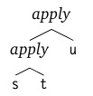
- Application (application or function call in relation to the given value) takes everything that it reaches. Those.
λx. λy. x y xmean the same asλx. (λy. ((x y) x))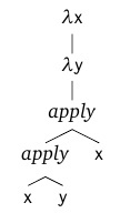
- The brackets explicitly indicate the grouping of actions.
It may seem like we need some special mechanisms for functions with several arguments, but in reality this is not so. Indeed, in the world of pure lambda calculus, the value returned by a function can also be a function. Therefore, we can apply the original function to only one of its arguments, “freezing” the others. As a result, we obtain a new function from the “tail” of arguments, to which the previous argument applies. This operation is called currying (in honor of the very Haskell Curry ). It will look something like this:
f = λx.λy.t | Function with two arguments xand yand bodyt |
f v w | Substitute the fvalues vandw |
(f v) w | This entry is similar to the previous one, but the parentheses clearly indicate the substitution sequence |
((λy.[x → v]t) w) | Framed vinstead x. [x → v]tmeans “body tin which all occurrences are xreplaced by v” |
[y → w][x → v]t | Framed winstead y. The conversion is complete. |
And finally, a few words about the scope . A variable
xis called bound if it is in the body of a tλ-abstraction λx.t. If it is xnot connected by any overlying abstraction, then it is called free . For example, the entries xin x yand are λy.x yfree, and the entries xin λx.xand λz.λx.λy.x(y z)are connected. The (λx.x)xfirst entry xis connected, and the second is free. If all the variables in the term are connected, then it is called closed , or combinator . We will use the following simple combinator ( identity function ):id = λx.x. It does not perform any action, but simply returns its argument without changes.Calculation process
Consider the following term application:
(λx.t) yIts left side
(λx.t)is a function with one argument xand a body t. Each step of the calculation will consist in replacing all occurrences of the variable xinside twith y. The term-application of this type is called redex (from reducible expression , redex - “abbreviated expression”), and the rewrite rewriting operation in accordance with this rule is called beta-reduction . There are several strategies for choosing a redex for the next calculation step. Treat them as an example, we will next term:
(λx.x) ((λx.x) (λz. (λx.x) z)), which for simplicity can be rewritten as
id (id (λz. id z))(recall that
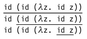
id Is a function of the identity of the species λx.x) This term contains three redexes:
- Complete β-reduction . In this case, each time the redex within the calculated term is chosen arbitrarily. Those. our example can be calculated from internal redex to external:
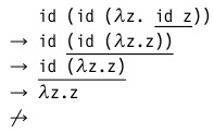
- Normal order of calculations . The first is always the leftmost, outermost redex.
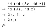
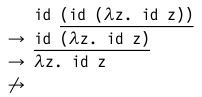
- Call by name . The calculation procedure in this strategy is similar to the previous one, but a ban on abbreviations inside the abstraction is added to it. Those. in our example, we stop at the penultimate step: An

optimized version of such a strategy (a call if necessary ) is used by Haskell. These are the so-called "lazy" calculations. - Call by value . Here the reduction begins with the leftmost (outer) redex, which has a value in the right-hand side - a closed term that cannot be calculated further.
For pure lambda calculus, such a term will be a λ-abstraction (function), and in richer calculi it can be constants, strings, lists, etc. This strategy is used in most programming languages when all arguments are computed first and then all are substituted into a function together.
If the term no longer has redexes, then they say that it is calculated , or is in normal form . Not every term has a normal form, for example,
(λx.xx)(λx.xx)at each step of the calculation it will generate itself (here the first bracket is an anonymous function, the second is the xvalue substituted into it ). The disadvantage of a value-based call strategy is that it may loop and not find the existing normal value of the term. For example, consider the expression
(λx.λy. x) z ((λx.x x)(λx.x x))This term has a normal form
zdespite the fact that his second argument does not have such a form. On its calculation, the call-by-value strategy will hang, while the call-by-name strategy will start from the outermost term and determine there that the second argument is not needed in principle. Conclusion: if the redex has a normal form, then the “lazy" strategy will definitely find it. Another subtlety is related to variable naming. For example, a term
(λx.λy.x)yafter substitution is calculated in λy.y. Those. due to the coincidence of variable names, we get an identity function where it was not originally intended. Indeed, we would call the local variable not y, but z- the original term would have the form (λx.λz.x)yand after reduction would have looked likeλz.y. To eliminate ambiguities of this kind, it is necessary to clearly monitor that all free variables from the initial term remain free after substitution. For this purpose, they use α-conversion - renaming a variable in abstraction in order to avoid name conflicts. It also happens that we have an abstraction
λx.t x, and it does not have xfree entries in the body t. In this case, this expression will be equivalently simple t. Such a transformation is called η-conversion . This concludes the introduction to the lambda calculus. In the next article, we will focus on what it was all about: programming on the λ-calculus.