Random Forest model for classification, implementation in c #
 Good day, reader. Random Forest today is one of the most popular and extremely effective methods for solving machine learning problems, such as classification and regression. In terms of efficiency, it competes with reference vector machines, neural networks and boosting, although it is certainly not without its drawbacks. In appearance, the learning algorithm is extremely simple (in comparison with, say, the learning machine algorithm of support vectors, who have little thrill in life, I highly recommend doing this at your leisure). We’ll try to understand in an accessible form the main ideas inherent in Random Forest (binary decision tree, bootstrap aggregation or bagging, random subspace method and decorrelation) and understand why all this works together. The model is quite young relative to its competitors: it all started with1997 article in which the authors proposed a method for constructing a single decision tree using the method of random subspaces of attributes when creating new tree nodes; then there was a series of articles, which culminated in the publication of a canonical version of the algorithm in 2001 , in which an ensemble of decision trees is built on the basis of bootstrap aggregation, or bagging. In the end, we will give a simple, not at all quick, but extremely visual way to implement this model in c #, as well as a series of tests. By the way, in the photo on the right you can see a real random forest that grows here in the Kaliningrad region on the Curonian Spit .
Binary decision tree
You should start with the tree, as with the main structural element of the forest, but in the context of the model under study. The presentation will be based on the assumption that the reader understands what a tree is like as a data structure . The tree will be constructed approximately according to the CART (Classification and Regression Tree) algorithm , which builds binary decision trees. By the way, here on the hub there is a suitable article on the construction of such trees based on minimizing entropy , in our version this will be a special case. So imagine a space of signs, let’s say two-dimensional, so that it would be easier to visualize, in which many objects of two classes are given.

We introduce a number of notation. We denote the set of signs as follows:
For each sign, we can distinguish the set of its values, either based on the training set, or using other a priori information about the problem, and denote the final set of values of the attribute as follows:
It is also necessary to introduce the so-called measure of the heterogeneity of the set with respect to its labels. Imagine that a subset of the training set consists of 5 red and 10 blue objects, then we can say that in this subset the probability of stretching the red object will be 1/3 , and the blue 2/3. Let us denote the probability of the kth class in a certain subset of the training set as follows:
Thus, we have defined the empirical discrete probability distribution of marks in the subset of observations. A measure of the heterogeneity of this subset will be called a function of the following form, where K (A) is the total number of labels of the subset A : The
measure of heterogeneity is set so that the value of the function increases as much as possible with increasing heterogeneity of the set, reaching its maximum when the set consists of the same the number of all kinds of labels, and the minimum if the set consists only of labels of one class (once again, I advise you to look at the entropy example with pictures)
Let's take a look at some examples of measures of heterogeneity (the vector p consists of m probabilities of labels found in some subset A of the training set):
- Most commonly occurring class:
- Gini index :
- Cross-entropy :
The algorithm for constructing the binary decision tree works according to the greedy algorithm : at each iteration, for the input subset of the training set, such a partition of space is constructed by a hyperplane (orthogonal to one of their coordinate axes) that would minimize the average measure of the heterogeneity of the two obtained subsets. This procedure is performed recursively for each subset received until stop criteria are met. We write it more formally, for the input set A we find the pair < sign , sign value >, that the measure of heterogeneity will be minimal:
where
 is the probability vector obtained by the above procedure from a subset of the set Aconsisting of those elements for which the condition f <x is fulfilled . Also, do not forget that the average cost of the partition should not exceed the cost of the original set. Let's go back to the original picture and take a look at what really happens, divide the original data set in the manner described above:
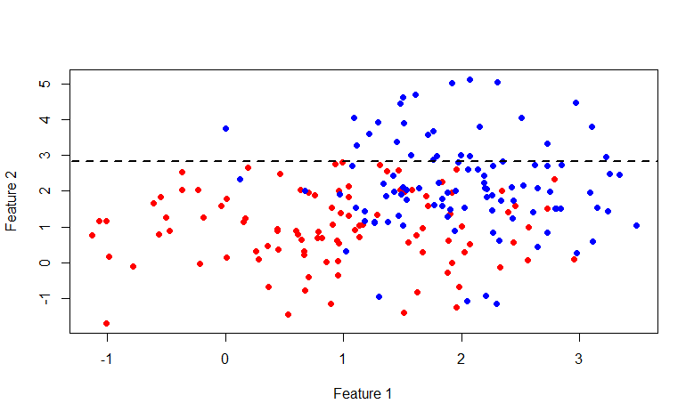
As you can see, the set above the line y = 2.840789 consists entirely of blue labels, so it makes sense to break down only the second set.
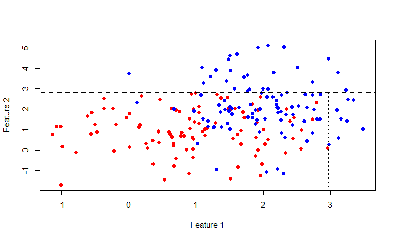
This time the line x = 2.976719 . In general, anyone interested in indulging in this picture, here is the R code:
Visualization code
rm(list=ls())
library(mvtnorm)
labCount <- 100
lab1 <- rmvnorm(n=labCount, mean=c(1,1), sigma=diag(c(1, 1)))
lab0 <- rmvnorm(n=labCount, mean=c(2,2), sigma=diag(c(0.5, 2)))
df <- data.frame(x=append(lab1[, 1], lab0[, 1]),
                 y=append(lab1[, 2], lab0[, 2]),
                 lab=append(rep(1, labCount), rep(0, labCount)))
plot(df$x, df$y, col=append(rep("red", labCount), rep("blue", labCount)), pch=19,
     xlab="Feature 1", ylab="Feature 2")
giniIdx <- function(data)
{
  p1 <- sum(data$lab == 1)/length(data$lab)
  p0 <- sum(data$lab == 0)/length(data$lab)
  return(p0*(1 - p0) + p1*(1 - p1))
}
p.norm <- giniIdx
getSeparator <- function(data)
{
  idx <- NA
  idx.val <- NA
  cost <- p.norm(data)
  for(i in 1:(dim(data)[2] - 1))
  {
    for(i.val in unique(data[, i]))
    {
      #print(paste("i = ", i, "; v = ", i.val, sep=""))
      cost.tmp <- 0.5*(p.norm(data[data[, i] < i.val, ]) +
                       p.norm(data[data[, i] >= i.val, ]))
      if(is.nan(cost.tmp))
      {
        next
      }
      if(cost.tmp < cost)
      {
        cost <- cost.tmp
        idx <- i
        idx.val <- i.val
      }
    }
  }
  return(c(idx, idx.val))
}
s1 <- getSeparator(df)
lines(c(-100, 100), c(s1[2], s1[2]), lty=2, lwd=2, type="l")
We list the possible stopping criteria: the maximum node depth has been reached; the probability of the dominant class in the partition exceeds a certain threshold (I use 0.95); the number of elements in the subset is less than a certain threshold. As a result, we get a partition of the whole set into (hyper) rectangles, and each such subset of the training set will be associated with one leaf of the tree, and all internal nodes are one of the conditions for the partition; or in other words some predicate. For the current node, the left child is associated with those elements of the set for which the predicate is true, and the right one, respectively, with the subject for which the predicate returns false. It looks like this:

So we got a tree, how can we make a decision on it? It will not be difficult for us to determine which of the subsets of the training set any input image belongs to, according to a particular decision tree. Next, we can only select the dominant class in this subset and return it to the client, or return the probability distribution of labels in this subset.
By the way, at the expense of the regression problem . The described method of constructing a tree easily changes from a classification problem to a regression task. For this, it is necessary to replace the measure of heterogeneity with some measure of forecasting error, for example, standard deviation. And when making a decision, instead of the dominant class, the average value of the target variable is used.
It seems that everything was decided with trees. We will not dwell on the pros and cons of this method; there is a good list on Wikipedia . But in the end, I want to add an illustration from the book An Introduction to Statistical Learning about the difference between linear models and trees.

This illustration shows the difference between a linear model and a binary decision tree, as you see in the case of linear separability, in general, the tree will show a less accurate result than a simple linear classifier.
Bootstrap aggregating or bagging
Let's move on to the next ideological component of random forest. So the name BAG ging is derived from B ootstrap AG gregating. In statistics, bootstrap is understood to mean both a method of estimating the standard error of statistics of a sample probability distribution and a method of sampling samples from a data set based on the Monte Carlo method .
Bootstrap sampling is pretty simple in its idea, and is used when we are not able to get a large number of samples from the real distribution, and this is almost always the case. Suppose we want to get m sets of observations of size n , but we have at our disposal only one set of nobservations. Then we generate m sets with an equiprobable choice of n elements from the original set with the return of the selected element ( selection with repetition or return ). For large values of n , the number of unique elements obtained by bootstrap by sampling the set will be (1 - 1 / e) ≈ 63.2% of the total number of unique observations of the initial set. Let D i - i -th set of received bootstrap sampling, we estimate it some parameter a i , and repeating this procedure mtime. The standard error bootstrap of parameter estimation is written as follows:
So, the statistical bootstrap allows estimating the error of estimation of some distribution parameter. But this is such a distraction from the topic, but we are interested in the bootstrap sampling method.
Now consider a set of m independent randomly selected elements x from one probability distribution, with some mathematical expectation and variance σ 2 . Then the sample average will be equal to:
The sample mean is not a distribution parameter, unlike the mean and variance, but a function of random variables, i.e. is also a random variable, from some probability distribution of sample means. And it, in turn, has the dispersion parameter, which is expressed as follows:
It turns out that averaging the set of values of a random variable reduces variability . This is the basis for the idea of aggregating bootstrap samples. We generate m bootstrap samples of size n from the training set D (also of size n ):

On each bootstrap sample, we train the model fand introduce the following function, this approach is called bootstrap aggregating or bagging:
Bagging can be illustrated by the following graph from Wikipedia , where the bag-model is shown by the red line and is an averaging of many other models.

Decorrelation
I think it’s already clear how to get just a forest: we generate a number of bootstrap samples and train the decision tree on each of them. But there is a small problem, almost all trees will be more or less the same structure. Let's do an experiment, take a set with two classes and 32 features , build 1000 decision trees on bootstrap samples, and look at the variability of the root node predicate.

We see that out of 1000 trees, the 22nd sign (obviously the value of the feature is the same) is found in 526 trees, and in almost all daughter nodes the same. In other words, the trees are correlatedrelative to each other. It turns out that it makes no sense to build 1000 trees, if only a few, and most often one or two, are enough. And now let's try when building a tree, when dividing each node, we use only some small random set of signs from the set of all signs, let's say 7 random from 32.

As you can see, the distribution has changed significantly towards a larger variety of trees (by the way, not only in the root node, but also in subsidiaries), which was the purpose of such a trick. Now 22 signs are found only in 158 cases. The choice of " 7 random out of 32 signs" is justified by an empirical observation (I have not found the author of this observation), and in classification problems this is usually the square root of the total number of signs.correlated , and the process is called decorrelation .
Such a method, in general, is called the Random subspace method and is used not only for decision trees, but also for other models, such as neural networks.
In general, something like this would look like an ordinary flat forest, and decorrelated.

Code
Let's move on to implementation. Once again, I want to remind you that the example I gave is not a quick implementation of random forest, but is only educational in nature, designed to help understand the main ideas of the model. For example, here you will find an example of a suitable and nimble implementation , but unfortunately less clear.
I will insert comments where necessary directly in the code, so as not to break the classes into pieces.
Ordinary tree
// обычное темплейт дерево, хотя конечно для бинарного дерева можно было бы сделать и проще publicclassTreeNode<T>
{
    publicTreeNode()
    {
        Childs = new LinkedList<TreeNode<T>>();
    }
    publicTreeNode(T data)
    {
        Data = data;
        Childs = new LinkedList<TreeNode<T>>();
    }
    public TreeNode<T> Parent { get; set; }
    public LinkedList<TreeNode<T>> Childs { get; set; }
    public T Data { get; set; }
    publicvirtualboolAddChild(T data)
    {
        TreeNode<T> node = new TreeNode<T>() {Data = data};
        node.Parent = this;
        Childs.AddLast(node);
        returntrue;
    }
    publicvirtualboolAddChild(TreeNode<T> node)
    {
        node.Parent = this;
        Childs.AddLast(node);
        returntrue;
    }
    publicbool IsLeaf
    {
        get
        {
            return Childs.Count == 0;
        }
    }
    publicint Depth
    {
        get
        {
            int d = 0;
            TreeNode<T> node = this;
            while (node.Parent != null)
            {
                d++;
                node = node.Parent;
            }
            return d;
        }
    }
}
The unit of observation in my case is represented by the following class.
Observation
publicclassDataItem<T>
{
    private T[] _input = null;
    private T[] _output = null;
    publicDataItem()
    {
    }
    publicDataItem(T[] input, T[] output)
    {
        _input = input;
        _output = output;
    }
    public T[] Input
    {
        get { return _input; }
        set { _input = value; }
    }
    public T[] Output
    {
        get { return _output; }
        set { _output = value; }
    }
}
For each node of the tree, it is necessary to store information about the predicate that is used to make a classification decision.
Tree Node Data
publicclassClassificationTreeNodeData
{
    // вектор вероятностей <id класса, его вероятность>, будем считать что он отсортирован по убыванию вероятностей// это то самое p из вышеприведенных формул первого разделаinternal IDictionary<double, double> Probabilities { get; set; }
    // стоимость данного узла, используется для того, что бы разбиение не было дороже текущей стоимости// чуть ниже мы представим это как норму вектораinternaldouble Cost { get; set; }
    // предикат который будет использоваться для принятия решения, полностью излишний элемент, // добавлен только ради эстетики, ведь мы не преследуем цель написать очень быстрый и экономный вариант -)internal Predicate<double[]> Predicate { get; set; }
    // данные ассоциированные с текущей нодой, используется только во время обучения дереваinternal IList<DataItem<double>> DataSet { get; set; }
    // имя ноды, используется при визуализации дереваinternalstring Name { get; set; }
    // индекс признака который минимизирует стоимость при разбиенииinternalint FeatureIndex { get; set; }
    // значение порога из области определения признакаinternaldouble FeatureValue { get; set; }
    // следующие две функции нужны изза того что дотнет не хочет сериализовать замыкания, которым является предикат
    [OnSerializing]
    privatevoidOnSerializing(StreamingContext context)
    {
        Predicate = null;
    }
    [OnDeserialized]
    [OnSerialized]
    privatevoidOnDeserialized(StreamingContext context)
    {
        Predicate = v => v[FeatureIndex] < FeatureValue;
    }
}
Consider the class of binary decision tree.
Binary decision tree
publicclassClassificationBinaryTree
{
    private TreeNode<ClassificationTreeNodeData> _rootNode = null;
    private INorm<double> _norm = null;     // норма вектора вероятностей privateint _minLeafDataCount = 1;    // минимально количество данных в наборе данных терминальной нодыprivateint[] _trainingFeaturesSubset = null;    // подмножество фичь которые могут участвовать в сплиттинге узла privateint _randomSubsetSize = 0;    // размер случайновыбираемых фич, как кандидатов при разделении нодыprivate Random _random = null;
    privatedouble _maxProbability = 0;     // максимальная вероятность класса, после достижения которой разделение ноды не происходитprivateint _maxDepth = Int32.MaxValue;     // максимальная глубина нодыprivatebool _showLog = false;
    privateint _featuresCount = 0;
    publicClassificationBinaryTree(INorm<double> norm, int minLeafDataCount, int[] trainingFeaturesSubset = null,
        int randomSubsetSize = 0, double maxProbability = 0.95, int maxDepth = Int32.MaxValue,
        bool showLog = false)
    {
        _norm = norm;
        _minLeafDataCount = minLeafDataCount;
        _trainingFeaturesSubset = trainingFeaturesSubset;
        _randomSubsetSize = randomSubsetSize;
        _maxProbability = maxProbability;
        _maxDepth = maxDepth;
        _showLog = showLog;
    }
    public TreeNode<ClassificationTreeNodeData> RootNode
    {
        get
        {
            return _rootNode;
        }
    }
    // обучение дереваpublicvoidTrain(IList<DataItem<double>> data)
    {
        _featuresCount = data.First().Input.Length;
        if (_randomSubsetSize > 0)
        {
            _random = new Random(Helper.GetSeed());
        }
        IDictionary<double, double> rootProbs = ComputeLabelsProbabilities(data);
        _rootNode = new TreeNode<ClassificationTreeNodeData>(new ClassificationTreeNodeData()
        {
            DataSet = data,
            Probabilities = rootProbs,
            Cost = _norm.Calculate(rootProbs.Select(x => x.Value).ToArray())
        });
        // не люблю рекурсии
        Queue<TreeNode<ClassificationTreeNodeData>> queue = new Queue<TreeNode<ClassificationTreeNodeData>>();
        queue.Enqueue(_rootNode);
        while (queue.Count > 0)
        {
            if (_showLog)
            {
                Logger.Instance.Log("Tree training: queue size is " + queue.Count);
            }
            TreeNode<ClassificationTreeNodeData> node = queue.Dequeue();
            int sourceCount = node.Data.DataSet.Count;
            // разделение ноды
            TrainNode(node, node.Data.DataSet, _trainingFeaturesSubset, _randomSubsetSize);
            if (_showLog && node.Childs.Count() > 0)
            {
                Logger.Instance.Log("Tree training: source " + sourceCount + " is splitted into " +
                                node.Childs.First().Data.DataSet.Count + " and " +
                                node.Childs.Last().Data.DataSet.Count);
            }
            // проверка остановки и продолжение роста дереваforeach (TreeNode<ClassificationTreeNodeData> child in node.Childs)
            {
                if (child.Data.Probabilities.Count == 1 ||
                    child.Data.DataSet.Count <= _minLeafDataCount ||
                    child.Data.Probabilities.First().Value > _maxProbability ||
                    child.Depth >= _maxDepth)
                {
                    child.Data.DataSet = null;
                    continue;
                }
                queue.Enqueue(child);
            }
        }
    }
    // разделение нодыprivatevoidTrainNode(TreeNode<ClassificationTreeNodeData> node, IList<DataItem<double>> data, int[] featuresSubset, int randomSubsetSize)
    {
        // argmin нормыdouble minCost = node.Data.Cost;
        int idx = -1;
        double threshold = 0;
        IDictionary<double, double> minLeftProbs = null;
        IDictionary<double, double> minRightProbs = null;
        IList<DataItem<double>> minLeft = null;
        IList<DataItem<double>> minRight = null;
        double minLeftCost = 0;
        double minRightCost = 0;
        // если требуется случайное подмножество фич, то заполняеif (randomSubsetSize > 0)
        {
            featuresSubset = newint[randomSubsetSize];
            IList<int> candidates = new List<int>();
            for (int i = 0; i < _featuresCount; i++)
            {
                candidates.Add(i);
            }
            for (int i = 0; i < randomSubsetSize; i++)
            {
                int idxRandom = _random.Next(0, candidates.Count);
                featuresSubset[i] = candidates[idxRandom];
                candidates.RemoveAt(idxRandom);
            }
        }
        elseif (featuresSubset == null)
        {
            featuresSubset = newint[data.First().Input.Length];
            for (int i = 0; i < data.First().Input.Length; i++)
            {
                featuresSubset[i] = i;
            }
        }
        // пробегаемся по выбранным признакамforeach (int i in featuresSubset)
        {
            IList<double> domain = data.Select(x => x.Input[i]).Distinct().ToList();
            // и ищем порог для минимизации стоимости разбиенияforeach (double t in domain)
            {
                IList<DataItem<double>> left = new List<DataItem<double>>(); // подмножество обучающего множества левого потомка
                IList<DataItem<double>> right = new List<DataItem<double>>(); // ну и правого
                IDictionary<double, double> leftProbs = new Dictionary<double, double>(); // вектор вероятностей классов в подмножестве
                IDictionary<double, double> rightProbs = new Dictionary<double, double>();
                foreach (DataItem<double> di in data)
                {
                    if (di.Input[i] < t)
                    {
                        left.Add(di);
                        if (!leftProbs.ContainsKey(di.Output[0]))
                        {
                            leftProbs.Add(di.Output[0], 0);
                        }
                        leftProbs[di.Output[0]]++;
                    }
                    else
                    {
                        right.Add(di);
                        if (!rightProbs.ContainsKey(di.Output[0]))
                        {
                            rightProbs.Add(di.Output[0], 0);
                        }
                        rightProbs[di.Output[0]]++;
                    }
                }
                if (right.Count == 0 || left.Count == 0)
                {
                    continue;
                }
                // нормализация вероятностей
                leftProbs = leftProbs.ToDictionary(x => x.Key, x => x.Value/left.Count);
                rightProbs = rightProbs.ToDictionary(x => x.Key, x => x.Value/right.Count);
                double leftCost = _norm.Calculate(leftProbs.Select(x => x.Value).ToArray());    // вычисление стоимости разбиения                           double rightCost = _norm.Calculate(rightProbs.Select(x => x.Value).ToArray());
                double avgCost = (leftCost + rightCost)/2;    // средняя стоимость разбиенияif (avgCost < minCost)
                {
                    minCost = avgCost;
                    idx = i;
                    threshold = t;
                    minLeftProbs = leftProbs;
                    minRightProbs = rightProbs;
                    minLeft = left;
                    minRight = right;
                    minLeftCost = leftCost;
                    minRightCost = rightCost;
                }
            }
        }
        // заполняем данные для текущей ноды и создаем потомков
        node.Data.DataSet = null;
        if (idx != -1)
        {
            //node should be splitted
            node.Data.Predicate = v => v[idx] < threshold;    // предикат который будет использоваться при принятии решений
            node.Data.Name = "x[" + idx + "] < " + threshold;
            node.Data.Probabilities = null;
            node.Data.FeatureIndex = idx;
            node.Data.FeatureValue = threshold;
            node.AddChild(new ClassificationTreeNodeData()
            {
                Probabilities = minLeftProbs.OrderByDescending(x => x.Value).ToDictionary(x => x.Key, x => x.Value),
                DataSet = minLeft,
                Cost = minLeftCost
            });
            node.AddChild(new ClassificationTreeNodeData()
            {
                Probabilities = minRightProbs.OrderByDescending(x => x.Value).ToDictionary(x => x.Key, x => x.Value),
                DataSet = minRight,
                Cost = minRightCost
            });
        }
    }
    // вычисление вероятностей классов в множестве, применяется в режиме классификацииprivate IDictionary<double, double> ComputeLabelsProbabilities(IList<DataItem<double>> data)
    {
        IDictionary<double, double> p = new Dictionary<double, double>();
        double denominator = data.Count;
        foreach (double label in data.Select(x => x.Output[0]).Distinct())
        {
            p.Add(label, data.Where(x => x.Output[0] == label).Count() / denominator);
        }
        return p;
    }
    // классификация вхожного образаpublic IDictionary<double, double> Classify(double[] v)
    {
        TreeNode<ClassificationTreeNodeData> node = _rootNode;
        while (!node.IsLeaf)
        {
            node = node.Data.Predicate(v) ? node.Childs.First() : node.Childs.Last();
        }
        return node.Data.Probabilities;
    }
    // запись дерева в формате GraphVis http://www.graphviz.org/publicvoidWriteDotFile(StreamWriter sw, bool separateTerminalNode = false)
    {
        sw.WriteLine("digraph G{");
        sw.WriteLine("graph [ordering=\"out\"];");
        Queue<TreeNode<ClassificationTreeNodeData>> q = new Queue<TreeNode<ClassificationTreeNodeData>>();
        q.Enqueue(_rootNode);
        int terminalCount = 0;
        ISet<string> styles = new HashSet<string>();
        while (q.Count > 0)
        {
            TreeNode<ClassificationTreeNodeData> node = q.Dequeue();
            foreach (TreeNode<ClassificationTreeNodeData> child in node.Childs)
            {
                string childName = child.Data.Name;
                if (String.IsNullOrEmpty(childName))
                {
                    if (separateTerminalNode)
                    {
                        childName = "TNode #" + terminalCount + "; Class: " + child.Data.Probabilities.First().Key;
                    }
                    else
                    {
                        childName = "Class: " + child.Data.Probabilities.First().Key;
                    }
                    styles.Add("\"" + childName + "\" [" +
                                "color=red, style=filled" +
                                "];");
                    terminalCount++;
                }
                sw.WriteLine("\"" + node.Data.Name + "\" -> " + "\"" + childName + "\";");
                q.Enqueue(child);
            }
        }
        foreach (string style in styles)
        {
            sw.WriteLine(style);
        }
        sw.WriteLine("}");
    }
}
Let us dwell on the norm used in the class of a decision tree.
Rate interface
publicinterfaceINorm<T>
{
    doubleCalculate(T[] v);
}
Gini Index
internalclassGiniIndex : INorm<double>
{
    #region INorm<double> MemberspublicdoubleCalculate(double[] v)
    {
        return v.Sum(p => p*(1 - p));
    }
    #endregion
}
Cross entropy
internalclassMetricsBasedNorm<T> : INorm<T>
{
    private IMetrics<T> _m = null;
    internalMetricsBasedNorm(IMetrics<T> m)
    {
        _m = m;
    }
    #region INorm<T> MemberspublicdoubleCalculate(T[] v)
    {
        return _m.Calculate(v, v);
    }
    #endregion
}
publicinterfaceIMetrics<T>
{
    ///<summary>/// Calculate value of metrics///</summary>doubleCalculate(T[] v1, T[] v2);
    ///<summary>/// Get centroid/clusteroid of data///</summary>T[] GetCentroid(IList<T[]> data);
    ///<summary>/// Calculate value of partial derivative by v2[v2Index]///</summary>T CalculatePartialDerivaitveByV2Index(T[] v1, T[] v2, int v2Index);
}
internalclassCrossEntropy : MetricsBase<double>
{
    internalCrossEntropy()
    {
    }
    ///<summary>/// \sum_i v1_i * ln(v2_i)///</summary>publicoverridedoubleCalculate(double[] v1, double[] v2)
    {
        if (v1.Length != v2.Length)
        {
            thrownew ArgumentException("Length of v1 and v2 should be equal");
        }
        if (v1.Length == 0 || v2.Length == 0)
        {
            thrownew ArgumentException("Vector dimension can't be 0");
        }
        double d = 0;
        for (int i = 0; i < v1.Length; i++)
        {
            d += v1[i]*Math.Log(v2[i] + Double.Epsilon);
        }
        return -d;
    }
    publicoverridedoubleCalculatePartialDerivaitveByV2Index(double[] v1, double[] v2, int v2Index)
    {
        return v2[v2Index] - v1[v2Index];
    }
}
Well, it remains to consider only the random forest class itself.
Random forest
publicclassClassificationRandomForest
{
    // параметры почти те же самые, добавился одинprivate INorm<double> _norm = null;
    privateint _minLeafDataCount = 1;
    privateint[] _trainingFeaturesSubset = null;
    privateint _randomSubsetSize = 0; //zero if all features neededprivatedouble _maxProbability = 0;
    privateint _maxDepth = Int32.MaxValue;
    privatebool _showLog = false;
    privateint _forestSize = 0;    // размер лесаprivate ConcurrentBag<ClassificationBinaryTree> _trees = null;
    publicClassificationRandomForest(INorm<double> norm, int forestSize, int minLeafDataCount, int[] trainingFeaturesSubset = null,
        int randomSubsetSize = 0, double maxProbability = 0.95, int maxDepth = Int32.MaxValue,
        bool showLog = false)
    {
        _norm = norm;
        _minLeafDataCount = minLeafDataCount;
        _trainingFeaturesSubset = trainingFeaturesSubset;
        _randomSubsetSize = randomSubsetSize;
        _maxProbability = maxProbability;
        _maxDepth = maxDepth;
        _forestSize = forestSize;
        _showLog = showLog;
    }
    publicvoidTrain(IList<DataItem<double>> data)
    {
        if (_showLog)
        {
            Logger.Instance.Log("Training is started");
        }
        // грех не распараллелить такое обучение, что бы каждое дерево росло самостоятельно
        _trees = new ConcurrentBag<ClassificationBinaryTree>();
        Parallel.For(0, _forestSize, i =>
        {
            ClassificationBinaryTree ct = new ClassificationBinaryTree(
                _norm,
                _minLeafDataCount,
                _trainingFeaturesSubset,
                _randomSubsetSize,
                _maxProbability,
                _maxDepth,
                false
                );
            ct.Train(BasicStatFunctions.Sample(data, data.Count, true));
            _trees.Add(ct);
            if (_showLog)
            {
                Logger.Instance.Log("Training of tree #" + _trees.Count + " is completed!");
            }
        });
    }
    // классификация, по сути это и есть baggingpublic IDictionary<double, double> Classify(double[] v)
    {
        IDictionary<double, double> p = new Dictionary<double, double>();
        foreach (ClassificationBinaryTree ct in _trees)
        {
            IDictionary<double, double> tr = ct.Classify(v);
            double winClass = tr.First().Key;
            if (!p.ContainsKey(winClass))
            {
                p.Add(winClass, 0);
            }
            p[winClass]++;
        }
        double denominator = p.Sum(x => x.Value);
        return
            p.ToDictionary(x => x.Key, x => x.Value/denominator)
                .OrderByDescending(x => x.Value)
                .ToDictionary(x => x.Key, x => x.Value);
    }
    public IList<ClassificationBinaryTree> Forest
    {
        get
        {
            return _trees.ToList();
        }
    }
}
Conclusion and references
If you looked into the code, you might notice that there is a function in the tree for writing the structure and conditions to the dot format, which is visualized by GraphVis . If you run a random forest with the following parameters on the above set :
ClassificationRandomForest crf = new ClassificationRandomForest(
        NormCreator.CreateByMetrics(MetricsCreator.CrossEntropy()),
        10,
        1,
        null,
        Convert.ToInt32(Math.Round(Math.Sqrt(ds.TrainSet.First().Input.Length))),
        0.95,
        1000,
        true
    );
crf.Train(ds.TrainSet);
Then the following code will help us visualize this forest:
foreach (ClassificationBinaryTree tree in crf.Forest)
{
    using (StreamWriter sw = new StreamWriter(@"e:\Neuroximator\NetworkTrainingOCR\TreeTestData\Forest\" +
            (new DirectoryInfo(@"e:\Neuroximator\NetworkTrainingOCR\TreeTestData\Forest\")).GetFiles().Count()
        + ".dot"))
    {
        tree.WriteDotFile(sw);
        sw.Close();
    }
}
dot.exe -Tpng "tree.dot" -o "tree.png"Let's look at some of them, they are completely different due to decorrelation.
Time

Two

Three

And finally, some useful links: