Analysis of the spherical motion of a solid in the Lagrange case
- From the sandbox
- Tutorial
This article will tell and show how to apply the Wolfram Mathematica environment to solving complex systems of differential equations, graphical interpretation of solution results, applying procedural programming elements to physical problems, using the example of a rigid body motion. The essence of the article is to show how, using computer algebra tools, it is easy and simple to analyze complex physical systems that excited the minds of 19th century physicists.
Spherical motion - the motion of a TT having one fixed point. Each of the points of the TT with this movement moves along the surface of the sphere with the center at the point of attachment. In this case, one speaks of rotational motion, which is composed of a series of elementary rotations around the instantaneous axes of rotation passing through the fixing point. The instantaneous axis of rotation continuously changes its position, both with respect to the reference frame in which the movement is considered, and in the body itself, thus forming two canonical surfaces, respectively called fixed and movable axoids.
TTwith a fixed point has 3 degrees of freedom, and its position with respect to this reference frame is determined by three parameters, and more precisely Euler angles. These angles define three turns of the system, which allow bringing any position of the system to the current.
If we take the elementary rotations of the SC around the axes Z and X in the order of Z, X ', Z' 'by the corresponding angles Ψ , θ, and φ , then this transformation leads to the expression of the rotation matrix in terms of Euler angles. Using such a matrix, the TT rotates in space.

The angles used have the following physical meaning:
The spherical motion of a TT , first described by Leonard Euler (German: Leonhard Euler), has a solution only in three cases:
Next, we will talk about the movement of a heavy symmetric top in the Lagrange case.
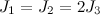
Let us draw a drawing of a heavy symmetric top in the field of gravity. We assign the role of the top to the cone.
We obtain the equations of motion from the kinetic moment theorem, having previously written it in general form in a movable SC .

Now we use the drawing we constructed and the theorem written down: omitting the tedious formulas, taking into account the moments of inertia of the symmetric top and presenting similar ones, we obtain the system of equations of motion of the TT in the field of gravity.
This system is not solved strictly analytically, and the solution is presented only in quadratures. We will solve this system numerically and analyze the results.
To begin with, we need to set the initial conditions for our remote control system :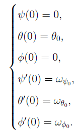
Next, using the capabilities of a computer algebra system, set the top parameters, draw primitives and solve the remote control system numerically .
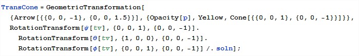
Then we get the rotation matrix, which we talked about earlier, using the built-in language tools, substitute the numerical solution there and apply the geometric transformation operator to this “cake”:
That's basically all the complexity of the solution in a couple of lines. It remains only to determine the graphic area, build a trajectory of motion and make an animation, but this is already, as they say to an amateur (you can limit yourself to the numerical derivation of transformation matrices). The rest of the code:
The output of the program results is carried out in the form of a window with dynamic parameters of the initial conditions of motion, animation time and transparency of the top.
Let us analyze the behavior of the top in the case of regular (forced) precession in the field of gravity:
According to the kinetic moment theorem (we talked about it above), for each small period of time dt, the angular momentum vector receives an increment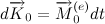 directed along the gravity along
 , i.e. lying in a horizontal plane perpendicular to the axis of the top. It follows that the vector of the angular momentum and with it the axis of the top rotate uniformly (precess) around a vertical line passing through the fulcrum. The top bent to the vertical precesses, i.e. in addition to rotation around its own axis, it also rotates around a vertical axis. With fast proper rotation, this precession (rotation around the vertical axis) occurs so slowly that with good accuracy we can neglect the component of the angular momentum that is caused by the precession around the vertical. This behavior of the top axis is called regular precession. This is a forced precession, since it occurs under the influence of the moment of gravity. All points of the top lying on its axis uniformly move along circular paths, the centers of which lie on the vertical passing through the fulcrum of the top. The illustration shows the regular precession of the top.
This event occurs only under strictly defined initial conditions.
Now we can proceed to study the question of how a spinning top will behave under the action of gravity under initial conditions that do not provide an immediate occurrence of a regular precession. In the general case, the motion of the top should be a superposition of forced regular precession and nutation, as shown in the figure.
At the first moment, as soon as we release the axis of the top, under the influence of gravity, it really begins to fall down, which is quite consistent with our intuitive ideas. But as the axis picks up speed, the trajectory of its upper end deviates more and more from the vertical. Soon, the movement of the axis becomes horizontal, as with a regular precession, but the speed of this movement is greater than what is needed for a regular precession. The trajectory of the end of the axis begins to deviate upward. Having risen to its original height, the axis "freezes" - its speed vanishes. Then everything repeats first. But now we understand what kind of behavior is, when the end of the axis moves along a cycloidal path,
When nutations are small, forced precession is called pseudo-regular, in the figure we can observe this phenomenon. For rapidly rotating gyroscopes (i.e., very fast rotating gyroscopes) used in technology, the pseudo-regular precession practically does not differ from the regular one. In such cases, nutation manifests itself as a barely noticeable small and frequent trembling of the axis of the gyroscope. In addition, small-scale nutations quickly decay under the action of friction forces, and the pseudo-regular precession becomes regular.
Thus, using such a powerful tool as Wolfram Mathematica, we can, without much effort and knowledge about programming, and most importantly intuitively, as classic textbooks suggest, observe interesting and mysterious processes and phenomena. The main thing is that we can independently twist and rotate any parameters of the system, which is very important for understanding. This project was my term paper, I sat on it for a couple of months, but I was pleased with the result. For a long time I twisted the animation of the motion of my top and played with the parameters observing various motion trajectories, which Lagrange or Kovalevskaya did not have.
upd. At the request of workers, I uploaded the project to DropBox.
Used Wolfram Mathematica 9.0
A bit about spherical motion
Spherical motion - the motion of a TT having one fixed point. Each of the points of the TT with this movement moves along the surface of the sphere with the center at the point of attachment. In this case, one speaks of rotational motion, which is composed of a series of elementary rotations around the instantaneous axes of rotation passing through the fixing point. The instantaneous axis of rotation continuously changes its position, both with respect to the reference frame in which the movement is considered, and in the body itself, thus forming two canonical surfaces, respectively called fixed and movable axoids.
TTwith a fixed point has 3 degrees of freedom, and its position with respect to this reference frame is determined by three parameters, and more precisely Euler angles. These angles define three turns of the system, which allow bringing any position of the system to the current.
Euler angles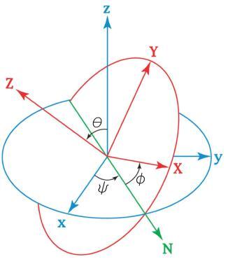
If we take the elementary rotations of the SC around the axes Z and X in the order of Z, X ', Z' 'by the corresponding angles Ψ , θ, and φ , then this transformation leads to the expression of the rotation matrix in terms of Euler angles. Using such a matrix, the TT rotates in space.
The angles used have the following physical meaning:
- Angle Ψ - angle of precession
- Angle θ - angle of nutation
- Angle φ - angle of proper rotation
The spherical motion of a TT , first described by Leonard Euler (German: Leonhard Euler), has a solution only in three cases:
- Euler's case - the center of mass of a TT , is at a fixed point. The moment of external forces is zero.
- The Lagrange - TT case is dynamically symmetric
 . The center of mass of the CT is on the axis of symmetry.
 - Kovalevskaya’s case - the body is dynamically symmetric, the moments of inertia are related by the relation
 . The center of mass of the TT is in the equatorial plane.
Next, we will talk about the movement of a heavy symmetric top in the Lagrange case.
The equations of motion in the case of Lagrange
Let us draw a drawing of a heavy symmetric top in the field of gravity. We assign the role of the top to the cone.
Picture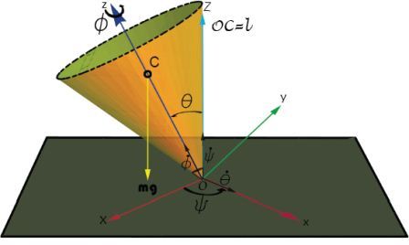
We obtain the equations of motion from the kinetic moment theorem, having previously written it in general form in a movable SC .
Now we use the drawing we constructed and the theorem written down: omitting the tedious formulas, taking into account the moments of inertia of the symmetric top and presenting similar ones, we obtain the system of equations of motion of the TT in the field of gravity.
This system is not solved strictly analytically, and the solution is presented only in quadratures. We will solve this system numerically and analyze the results.
Modeling the Lagrange case in the Wolfram Mathematica system
To begin with, we need to set the initial conditions for our remote control system :
Next, using the capabilities of a computer algebra system, set the top parameters, draw primitives and solve the remote control system numerically .
Code snippets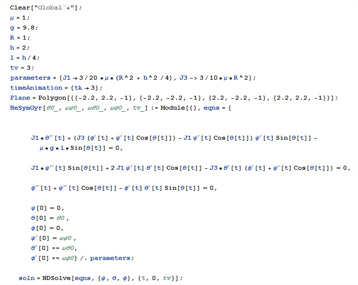
Then we get the rotation matrix, which we talked about earlier, using the built-in language tools, substitute the numerical solution there and apply the geometric transformation operator to this “cake”:
That's basically all the complexity of the solution in a couple of lines. It remains only to determine the graphic area, build a trajectory of motion and make an animation, but this is already, as they say to an amateur (you can limit yourself to the numerical derivation of transformation matrices). The rest of the code:
The rest of
Conclusion and analysis of results in the Wolfram Mathematica system
The output of the program results is carried out in the form of a window with dynamic parameters of the initial conditions of motion, animation time and transparency of the top.
Let us analyze the behavior of the top in the case of regular (forced) precession in the field of gravity:
According to the kinetic moment theorem (we talked about it above), for each small period of time dt, the angular momentum vector receives an increment
directed along the gravity along, i.e. lying in a horizontal plane perpendicular to the axis of the top. It follows that the vector of the angular momentum and with it the axis of the top rotate uniformly (precess) around a vertical line passing through the fulcrum. The top bent to the vertical precesses, i.e. in addition to rotation around its own axis, it also rotates around a vertical axis. With fast proper rotation, this precession (rotation around the vertical axis) occurs so slowly that with good accuracy we can neglect the component of the angular momentum that is caused by the precession around the vertical. This behavior of the top axis is called regular precession. This is a forced precession, since it occurs under the influence of the moment of gravity. All points of the top lying on its axis uniformly move along circular paths, the centers of which lie on the vertical passing through the fulcrum of the top. The illustration shows the regular precession of the top.Regular precession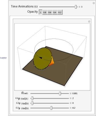
This event occurs only under strictly defined initial conditions.
Now we can proceed to study the question of how a spinning top will behave under the action of gravity under initial conditions that do not provide an immediate occurrence of a regular precession. In the general case, the motion of the top should be a superposition of forced regular precession and nutation, as shown in the figure.
General case of movement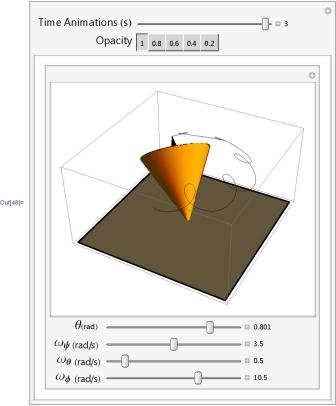
At the first moment, as soon as we release the axis of the top, under the influence of gravity, it really begins to fall down, which is quite consistent with our intuitive ideas. But as the axis picks up speed, the trajectory of its upper end deviates more and more from the vertical. Soon, the movement of the axis becomes horizontal, as with a regular precession, but the speed of this movement is greater than what is needed for a regular precession. The trajectory of the end of the axis begins to deviate upward. Having risen to its original height, the axis "freezes" - its speed vanishes. Then everything repeats first. But now we understand what kind of behavior is, when the end of the axis moves along a cycloidal path,
When nutations are small, forced precession is called pseudo-regular, in the figure we can observe this phenomenon. For rapidly rotating gyroscopes (i.e., very fast rotating gyroscopes) used in technology, the pseudo-regular precession practically does not differ from the regular one. In such cases, nutation manifests itself as a barely noticeable small and frequent trembling of the axis of the gyroscope. In addition, small-scale nutations quickly decay under the action of friction forces, and the pseudo-regular precession becomes regular.
Pseudo-regular precession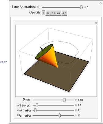
Conclusion
Thus, using such a powerful tool as Wolfram Mathematica, we can, without much effort and knowledge about programming, and most importantly intuitively, as classic textbooks suggest, observe interesting and mysterious processes and phenomena. The main thing is that we can independently twist and rotate any parameters of the system, which is very important for understanding. This project was my term paper, I sat on it for a couple of months, but I was pleased with the result. For a long time I twisted the animation of the motion of my top and played with the parameters observing various motion trajectories, which Lagrange or Kovalevskaya did not have.
Literature
- Wittenburg, J. Dynamics of solids / J. Wittenburg.- Moscow: MIR, 1980.-294 p.:
- Rotational motion.
- Euler angles.
- Forced gyroscope precession.
upd. At the request of workers, I uploaded the project to DropBox.
Used Wolfram Mathematica 9.0