Writing XGBoost from scratch - part 2: gradient boosting

Tutorial

Hello!

In the last article, we figured out how the decisive trees are arranged, and implemented
the construction algorithm from scratch , simultaneously optimizing and improving it. In this article, we will implement a gradient boost algorithm and at the end create our own XGBoost. The narration will follow the same pattern: we write an algorithm, describe it, summarize the results, comparing the results of work with analogues from Sklearn.

In this article, the emphasis will also be made on the implementation in the code, so the whole theory is better read in another together (for example, in the ODS course ), and already with the knowledge of the theory, you can move on to this article, since the topic is quite complicated.

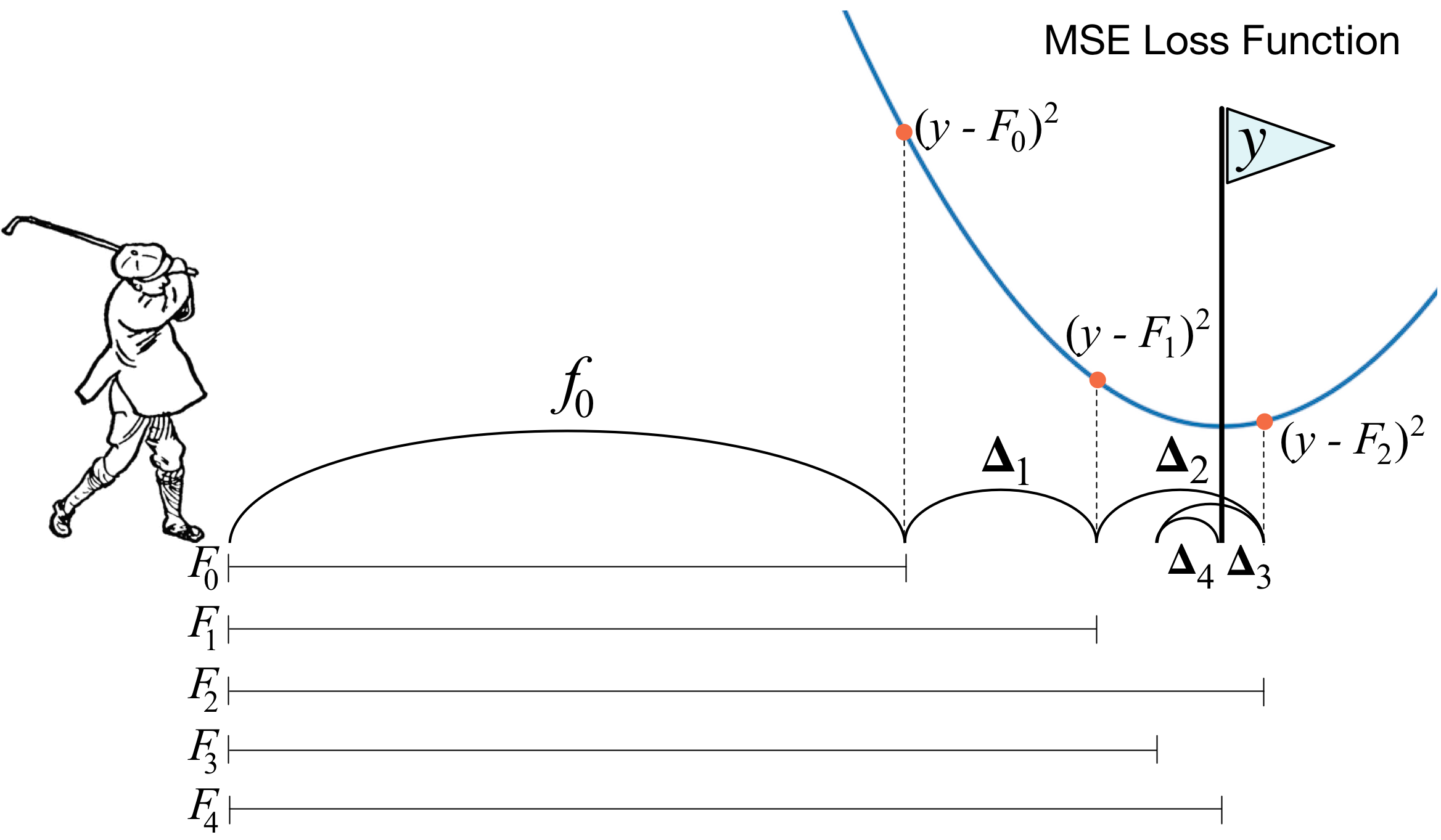
What is gradient boosting? A picture with a golfer best describes the main idea. In order to drive the ball into the hole, the golfer makes every next strike, taking into account the experience of previous shots - for him it is a necessary condition to drive the ball into the hole. If it’s very rough (I’m not a master of the game of golf :)), then with each new strike the first thing a golfer looks at is the distance between the ball and the hole after the previous strike. And the main task is to reduce this distance with the next blow.

Boosting is built in a very similar way. First, we need to introduce the definition of "hole", that is, the goal to which we will strive. Secondly, we need to learn to understand which way to hit with a club in order to get closer to the goal. Thirdly, taking into account all these rules, you need to come up with the correct sequence of blows, so that each subsequent one shortens the distance between the ball and the hole.

Now we give a slightly more rigorous definition. We introduce a weighted voting model:

$h (x) = \ sum_ {i = 1} ^ nb_ia_i, x \ in X, b_i \ in R$

Here

$inline$ Is the space from which we take objects

$inline$ - this is the coefficient in front of the model and the model itself, that is, the decision tree. Suppose that already at some step, using the described rules, we managed to add to the composition

$inline$ weak algorithm. To learn to understand what exactly the algorithm should be on the step

$inline$ , we introduce the error function:

$err (h) = \ sum_ {j = 1} ^ NL (\ sum_ {i = 1} ^ {T-1} a_ib_i (x_j) + b_Ta_T (x_j)) \ rightarrow min_ {a_T, b_T}$

It turns out that the best algorithm is the one that can minimize the error obtained at previous iterations. And since the boosting is gradient, then this error function must necessarily have an anti-gradient vector along which you can move in search of a minimum. Everything!

Immediately before the implementation I will insert a few words about how exactly everything will be arranged. As in the previous article, let's take MSE as a loss. Calculate its gradient:

$mse (y, predict) = (y - predict) ^ 2 \\ \ nabla_ {predict} mse (y, predict) = predict - y$

Thus, the antigradient vector will be equal to

$inline$ . On the move

$inline$ we consider the errors of the algorithm obtained at past iterations. Next, we train our new algorithm on these errors, and then with a minus sign and add some coefficient to our ensemble.

Now we will start implementation.

1. Implement the usual gradient boost class

import pandas as pd
import matplotlib.pyplot as plt
import numpy as np
from tqdm import tqdm_notebook
from sklearn import datasets
from sklearn.metrics import mean_squared_error as mse
from sklearn.tree import DecisionTreeRegressor
import itertools
%matplotlib inline
%load_ext Cython
%%cython -a 
import itertools
import numpy as np
cimport numpy as np
from itertools import *
cdef classRegressionTreeFastMse:
    cdef public int max_depth
    cdef public int feature_idx
    cdef public int min_size
    cdef public int averages 
    cdef public np.float64_t feature_threshold
    cdef public np.float64_t value
    cpdef RegressionTreeFastMse left
    cpdef RegressionTreeFastMse right
    def__init__(self, max_depth=3, min_size=4, averages=1):
        self.max_depth = max_depth
        self.min_size = min_size
        self.value = 0
        self.feature_idx = -1
        self.feature_threshold = 0
        self.left = None
        self.right = Nonedeffit(self, np.ndarray[np.float64_t, ndim=2] X, np.ndarray[np.float64_t, ndim=1] y):
        cpdef np.float64_t mean1 = 0.0
        cpdef np.float64_t mean2 = 0.0
        cpdef long N = X.shape[0]
        cpdef long N1 = X.shape[0]
        cpdef long N2 = 0
        cpdef np.float64_t delta1 = 0.0
        cpdef np.float64_t delta2 = 0.0
        cpdef np.float64_t sm1 = 0.0
        cpdef np.float64_t sm2 = 0.0
        cpdef list index_tuples
        cpdef list stuff
        cpdef long idx = 0
        cpdef np.float64_t prev_error1 = 0.0
        cpdef np.float64_t prev_error2 = 0.0
        cpdef long thres = 0
        cpdef np.float64_t error = 0.0
        cpdef np.ndarray[long, ndim=1] idxs
        cpdef np.float64_t x = 0.0# начальное значение - среднее значение y
        self.value = y.mean()
        # начальная ошибка - mse между значением в листе 
        base_error = ((y - self.value) ** 2).sum()
        error = base_error
        flag = 0# пришли на максимальную глубинуif self.max_depth <= 1:
            return
        dim_shape = X.shape[1]
        left_value, right_value = 0, 0for feat in range(dim_shape):
            prev_error1, prev_error2 = base_error, 0 
            idxs = np.argsort(X[:, feat])
            # переменные для быстрого переброса суммы
            mean1, mean2 = y.mean(), 0
            sm1, sm2 = y.sum(), 0
            N = X.shape[0]
            N1, N2 = N, 0
            thres = 1while thres < N - 1:
                N1 -= 1
                N2 += 1
                idx = idxs[thres]
                x = X[idx, feat]
                # вычисляем дельты - по ним, в основном, будет делаться переброс
                delta1 = (sm1 - y[idx]) * 1.0 / N1 - mean1
                delta2 = (sm2 + y[idx]) * 1.0 / N2 - mean2
                # увеличиваем суммы
                sm1 -= y[idx]
                sm2 += y[idx]
                # пересчитываем ошибки за O(1)
                prev_error1 += (delta1**2) * N1 
                prev_error1 -= (y[idx] - mean1)**2 
                prev_error1 -= 2 * delta1 * (sm1 - mean1 * N1)
                mean1 = sm1/N1
                prev_error2 += (delta2**2) * N2 
                prev_error2 += (y[idx] - mean2)**2 
                prev_error2 -= 2 * delta2 * (sm2 - mean2 * N2)
                mean2 = sm2/N2
                # пропускаем близкие друг к другу значенияif thres < N - 1and np.abs(x - X[idxs[thres + 1], feat]) < 1e-5:
                    thres += 1continueif (prev_error1 + prev_error2 < error):
                    if (min(N1,N2) > self.min_size):
                        # переопределяем самый лучший признак и границу по нему
                        self.feature_idx, self.feature_threshold = feat, x
                        # переопределяем значения в листах
                        left_value, right_value = mean1, mean2
                        # флаг - значит сделали хороший сплит
                        flag = 1
                        error = prev_error1 + prev_error2
                thres += 1# ничего не разделили, выходимif self.feature_idx == -1:
            return# вызываем потомков дерева
        self.left = RegressionTreeFastMse(self.max_depth - 1)
        self.left.value = left_value
        self.right = RegressionTreeFastMse(self.max_depth - 1)
        self.right.value = right_value
        # новые индексы для обучения потомков
        idxs_l = (X[:, self.feature_idx] > self.feature_threshold)
        idxs_r = (X[:, self.feature_idx] <= self.feature_threshold)
        # обучение потомков
        self.left.fit(X[idxs_l, :], y[idxs_l])
        self.right.fit(X[idxs_r, :], y[idxs_r])
    def__predict(self, np.ndarray[np.float64_t, ndim=1] x):if self.feature_idx == -1:
            return self.value
        if x[self.feature_idx] > self.feature_threshold:
            return self.left.__predict(x)
        else:
            return self.right.__predict(x)
    defpredict(self, np.ndarray[np.float64_t, ndim=2] X):
        y = np.zeros(X.shape[0])
        for i in range(X.shape[0]):
            y[i] = self.__predict(X[i])
        return y

classGradientBoosting():def__init__(self, n_estimators=100, learning_rate=0.1, max_depth=3, 
                 random_state=17, n_samples = 15, min_size = 5, base_tree='Bagging'):
        self.n_estimators = n_estimators
        self.max_depth = max_depth
        self.learning_rate = learning_rate
        self.initialization = lambda y: np.mean(y) * np.ones([y.shape[0]])
        self.min_size = min_size
        self.loss_by_iter = []
        self.trees_ = []
        self.loss_by_iter_test = []
        self.n_samples = n_samples
        self.base_tree = base_tree
    deffit(self, X, y):
        self.X = X
        self.y = y
        b = self.initialization(y)
        prediction = b.copy()
        for t in tqdm_notebook(range(self.n_estimators)):               
            if t == 0:
                resid = y
            else:
                # сразу пишем антиградиент
                resid = (y - prediction)
            # выбираем базовый алгоритмif self.base_tree == 'Bagging':
                tree = Bagging(max_depth=self.max_depth,
                                       min_size = self.min_size)                
            if self.base_tree == 'Tree':
                tree = RegressionTreeFastMse(max_depth=self.max_depth,
                                          min_size = self.min_size)
            # обучаемся на векторе антиградиента
            tree.fit(X, resid)
            # делаем предикт и добавляем алгоритм к ансамблю
            b = tree.predict(X).reshape([X.shape[0]])
            self.trees_.append(tree)
            prediction += self.learning_rate * b
            # добавляем только если не первая итерацияif t > 0:
                self.loss_by_iter.append(mse(y,prediction))
        return self
    defpredict(self, X):# сначала прогноз – это просто вектор из средних значений ответов на обучении
        pred = np.ones([X.shape[0]]) * np.mean(self.y)
        # добавляем прогнозы деревьевfor t in range(self.n_estimators):
            pred += self.learning_rate * self.trees_[t].predict(X).reshape([X.shape[0]])
        return pred

We now construct the loss curve on the training set to make sure that with each iteration we actually have its decrease.

GDB = GradientBoosting(n_estimators=50)
GDB.fit(X,y)
x = GDB.predict(X)
plt.grid()
plt.title('Loss by iterations')
plt.plot(GDB.loss_by_iter)

2. Bagging over decisive trees

Well, before we compare the results, let's talk more about the procedure of beggling over the trees.

Everything is simple here: we want to protect ourselves from retraining, and therefore, with the help of return samples, we will average our predictions in order not to accidentally run into emissions (why it works like this - read the link better).

classBagging():'''
    Класс Bagging - предназначен для генерирования бустрапированного
    выбора моделей.
    '''def__init__(self, max_depth = 3, min_size=10, n_samples = 10):#super(CART, self).__init__()
        self.max_depth = max_depth
        self.min_size = min_size
        self.n_samples = n_samples
        self.subsample_size = None
        self.list_of_Carts = [RegressionTreeFastMse(max_depth=self.max_depth, 
                                min_size=self.min_size) for _ in range(self.n_samples)]
    defget_bootstrap_samples(self, data_train, y_train):# генерируем индексы выборок с возращением
        indices = np.random.randint(0, len(data_train), (self.n_samples, self.subsample_size))
        samples_train = data_train[indices]
        samples_y = y_train[indices]
        return samples_train, samples_y
    deffit(self, data_train, y_train):# обучаем каждую модель 
        self.subsample_size = int(data_train.shape[0])
        samples_train, samples_y = self.get_bootstrap_samples(data_train, y_train)
        for i in range(self.n_samples):
            self.list_of_Carts[i].fit(samples_train[i], samples_y[i].reshape(-1))
        return self
    defpredict(self, test_data):# для каждого объекта берём его средний предикт
        num_samples = test_data.shape[0]
        pred = []
        for i in range(self.n_samples):
            pred.append(self.list_of_Carts[i].predict(test_data))
        pred = np.array(pred).T
        return np.array([np.mean(pred[i]) for i in range(num_samples)])

Great, now we can use not one tree as the base algorithm, but tree begging - so, again, we will defend against retraining.

3. Results

Compare the results of our algorithms.

from sklearn.model_selection import KFold
import matplotlib.pyplot as plt
from sklearn.ensemble import GradientBoostingRegressor as GDBSklearn
import copy
defget_metrics(X,y,n_folds=2, model=None):
    kf = KFold(n_splits=n_folds, shuffle=True)
    kf.get_n_splits(X)
    er_list = []
    for train_index, test_index in tqdm_notebook(kf.split(X)):
        X_train, X_test = X[train_index], X[test_index]
        y_train, y_test = y[train_index], y[test_index]
        model.fit(X_train,y_train)
        predict = model.predict(X_test)
        er_list.append(mse(y_test, predict))
    return er_list
data = datasets.fetch_california_housing()
X = np.array(data.data)
y = np.array(data.target)
er_boosting = get_metrics(X,y,30,GradientBoosting(max_depth=3, n_estimators=40, base_tree='Tree' ))
er_boobagg = get_metrics(X,y,30,GradientBoosting(max_depth=3, n_estimators=40, base_tree='Bagging' ))
er_sklearn_boosting = get_metrics(X,y,30,GDBSklearn(max_depth=3,n_estimators=40, learning_rate=0.1))
%matplotlib inline
data = [er_sklearn_boosting, er_boosting, er_boobagg]
fig7, ax7 = plt.subplots()
ax7.set_title('')
ax7.boxplot(data, labels=['Sklearn Boosting', 'Boosting', 'BooBag'])
plt.grid()
plt.show()

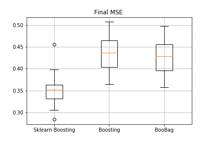
Received:

We can not yet beat the equivalent of Sklearn, because again we do not take into account a lot of parameters that are used in this method . However, we see that bagging helps a bit.

Let's not despair, and move on to writing XGBoost'a.

4. XGBoost

Before reading further, I strongly advise you first to familiarize yourself with the following video , the theory is very well explained in it.

Recall what error we minimize in the usual boosting:

$err (h) = \ sum_ {j = 1} ^ NL (\ sum_ {i = 1} ^ {T-1} a_ib_i (x_j) + b_Ta_T (x_j))$

XGBoost explicitly adds regularization to this error functionality:

$err (h) = \ sum_ {j = 1} ^ NL (\ sum_ {i = 1} ^ {T-1} a_ib_i (x_j) + b_Ta_T (x_j)) + \ sum_ {i = 1} ^ T \ omega (a_i)$

How to count this functionality? First, we bring it closer with the help of the second-order Taylor series, where the new algorithm is considered as an increment along which we will move, and we will write further on depending on the loss we have:

$f (x + \ delta x) \ thickapprox f (x) + f (x) '\ delta x + 0.5 * f (x)' '(\ delta x) ^ 2$

It is necessary to determine which tree we will consider bad and which one to be good.

Recall the principle on which the regression with

$inline$ -regularization - the more normal values of the coefficients before regression, the worse, so you need to be as small as possible.

In XGBoost, the idea is very similar: a tree is penalized if the sum of the norm values in the leaves in it is very large. Therefore, the complexity of the tree is introduced here as follows:

$\ omega (a) = \ gamma Z + 0.5 * \ sum_ {i = 1} ^ {Z} w_i ^ 2$

$inline$ - values in the leaves,

$inline$ - the number of leaves.

There are transitional formulas in the video, we will not display them here. It all comes down to the fact that we will choose the new partition, maximizing the gain:

$Gain = \ frac {G_l ^ 2} {S_l ^ 2 + \ lambda} + \ frac {G_r ^ 2} {S_r ^ 2 + \ lambda} - \ frac {(G_l + G_r) ^ 2} {S_l ^ 2 + S_r ^ 2 + \ lambda} - \ gamma$

Here

$\ gamma, \ lambda$ Are the numerical parameters of the regularization, and

$inline$ - the corresponding amounts of the first and second derivatives for this partition.

Everything, the theory is very briefly stated, the links are given, now let's talk about what the derivatives will be if we work with MSE. It's simple:

$mse (y, predict) = (y - predict) ^ 2 \\ \ nabla_ {predict} mse (y, predict) = predict - y \\ \ nabla_ {predict} ^ 2 mse (y, predict) = 1$

When will we take the amount

$inline$ , just add to the first

$inline$ , and to the second - just the amount.

%%cython -a 
import numpy as np
cimport numpy as np
cdef classRegressionTreeGain:
    cdef public int max_depth
    cdef public np.float64_t gain
    cdef public np.float64_t lmd
    cdef public np.float64_t gmm
    cdef public int feature_idx
    cdef public int min_size
    cdef public np.float64_t feature_threshold
    cdef public np.float64_t value
    cpdef public RegressionTreeGain left
    cpdef public RegressionTreeGain right
    def__init__(self, int max_depth=3, np.float64_t lmd=1.0, np.float64_t gmm=0.1, min_size=5):
        self.max_depth = max_depth
        self.gmm = gmm
        self.lmd = lmd
        self.left = None
        self.right = None
        self.feature_idx = -1
        self.feature_threshold = 0
        self.value = -1e9
        self.min_size = min_size
        returndeffit(self, np.ndarray[np.float64_t, ndim=2] X, np.ndarray[np.float64_t, ndim=1] y):
        cpdef long N = X.shape[0]
        cpdef long N1 = X.shape[0]
        cpdef long N2 = 0
        cpdef long idx = 0
        cpdef long thres = 0
        cpdef np.float64_t gl, gr, gn
        cpdef np.ndarray[long, ndim=1] idxs
        cpdef np.float64_t x = 0.0
        cpdef np.float64_t best_gain = -self.gmm
        if self.value == -1e9:
            self.value = y.mean()
        base_error = ((y - self.value) ** 2).sum()
        error = base_error
        flag = 0if self.max_depth <= 1:
            return
        dim_shape = X.shape[1]
        left_value = 0
        right_value = 0# начинаем процесс обучения# чуть-чуть матана - у нас mse, L = (y - pred)**2# dL/dpred = pred - y, эту разницу мы в бустинге будем передавать со знаком -# dL^2/d^2pred = 1 - получается, это просто количество объектов в листеfor feat in range(dim_shape):
            idxs = np.argsort(X[:, feat])
            gl,gr = y.sum(),0.0
            N1, N2, thres = N, 0, 0while thres < N - 1:
                N1 -= 1
                N2 += 1
                idx = idxs[thres]
                x = X[idx, feat]
                gl -= y[idx]
                gr += y[idx]
                # считаем гейн
                gn = (gl**2) / (N1 + self.lmd)  + (gr**2) / (N2 + self.lmd)
                gn -= ((gl + gr)**2) / (N1 + N2 + self.lmd) + self.gmm
                if thres < N - 1and x == X[idxs[thres + 1], feat]:
                    thres += 1continue# проверяем условия на гейнif (gn > best_gain) and (min(N1,N2) > self.min_size):
                    flag = 1
                    best_gain = gn
                    left_value = -gl / (N1 + self.lmd)
                    right_value = -gr / (N2 + self.lmd)
                    self.feature_idx = feat
                    self.feature_threshold = x
                thres += 1
        self.gain = best_gain
        if self.feature_idx == -1:
            return
        self.left = RegressionTreeGain(max_depth=self.max_depth - 1, gmm=self.gmm, lmd=self.lmd)
        self.left.value = left_value
        self.right = RegressionTreeGain(max_depth=self.max_depth - 1, gmm=self.gmm, lmd=self.lmd)
        self.right.value = right_value
        idxs_l = (X[:, self.feature_idx] > self.feature_threshold)
        idxs_r = (X[:, self.feature_idx] <= self.feature_threshold)
        self.left.fit(X[idxs_l, :], y[idxs_l])
        self.right.fit(X[idxs_r, :], y[idxs_r])
        # подрубаем отрицательный гейнif (self.left.left == Noneor self.right.left == None):
            if self.gain < 0.0:
                self.left = None
                self.right = None
                self.feature_idx = -1def__predict(self, np.ndarray[np.float64_t, ndim=1] x):if self.feature_idx == -1:
            return self.value
        if x[self.feature_idx] > self.feature_threshold:
             return self.left.__predict(x)
        else:
            return self.right.__predict(x)
    defpredict(self, np.ndarray[np.float64_t, ndim=2] X):
        y = np.zeros(X.shape[0])
        for i in range(X.shape[0]):
            y[i] = self.__predict(X[i])
        return y

A small clarification: so that the formulas in the trees with a gain were more beautiful, in the boosting we train the target with a minus sign.

Slightly modify our boosting, make some parameters adaptive. For example, if we notice that the loss has begun to emerge on a plateau, then we decrease the learning rate and increase the max_depth for the following estimators. We will also add a new bagging - now we will make a boosting over the baggings from trees with a gain:

classBagging():def__init__(self, max_depth = 3, min_size=5, n_samples = 10):
        self.max_depth = max_depth
        self.min_size = min_size
        self.n_samples = n_samples
        self.subsample_size = None
        self.list_of_Carts = [RegressionTreeGain(max_depth=self.max_depth, 
                                min_size=self.min_size) for _ in range(self.n_samples)]
    defget_bootstrap_samples(self, data_train, y_train):
        indices = np.random.randint(0, len(data_train), (self.n_samples, self.subsample_size))
        samples_train = data_train[indices]
        samples_y = y_train[indices]
        return samples_train, samples_y
    deffit(self, data_train, y_train):
        self.subsample_size = int(data_train.shape[0])
        samples_train, samples_y = self.get_bootstrap_samples(data_train, y_train)
        for i in range(self.n_samples):
            self.list_of_Carts[i].fit(samples_train[i], samples_y[i].reshape(-1))
        return self
    defpredict(self, test_data):
        num_samples = test_data.shape[0]
        pred = []
        for i in range(self.n_samples):
            pred.append(self.list_of_Carts[i].predict(test_data))
        pred = np.array(pred).T
        return np.array([np.mean(pred[i]) for i in range(num_samples)])

classGradientBoosting():def__init__(self, n_estimators=100, learning_rate=0.2, max_depth=3, 
                 random_state=17, n_samples = 15, min_size = 5, base_tree='Bagging'):
        self.n_estimators = n_estimators
        self.max_depth = max_depth
        self.learning_rate = learning_rate
        self.initialization = lambda y: np.mean(y) * np.ones([y.shape[0]])
        self.min_size = min_size
        self.loss_by_iter = []
        self.trees_ = []
        self.loss_by_iter_test = []
        self.n_samples = n_samples
        self.base_tree = base_tree
        # хотим как-то регулировать работу алгоритма на поздних итерациях# если ошибка застряла, то уменьшаем lr и увеличиваем max_depth
        self.add_to_max_depth = 1
        self.init_mse_board = 1.5deffit(self, X, y):print (self.base_tree)
        self.X = X
        self.y = y
        b = self.initialization(y)
        prediction = b.copy()
        for t in tqdm_notebook(range(self.n_estimators)):
            if t == 0:
                resid = y
            else:
                resid = (y - prediction)
                if (mse(temp_resid,resid) < self.init_mse_board):
                    self.init_mse_board /= 1.5
                    self.add_to_max_depth += 1
                    self.learning_rate /= 1.1# print ('Alert!', t, self.add_to_max_depth)if self.base_tree == 'Bagging':
                tree = Bagging(max_depth=self.max_depth+self.add_to_max_depth,
                                         min_size = self.min_size)
                resid = -resid
            if self.base_tree == 'Tree':
                tree = RegressionTreeFastMse(max_depth=self.max_depth+self.add_to_max_depth, min_size = self.min_size)
            if self.base_tree == 'XGBoost':
                tree = RegressionTreeGain(max_depth=self.max_depth+self.add_to_max_depth, min_size = self.min_size)
                resid = -resid
            tree.fit(X, resid)
            b = tree.predict(X).reshape([X.shape[0]])
            # print (b.shape)
            self.trees_.append(tree)
            prediction += self.learning_rate * b
            temp_resid = resid
        return self
    defpredict(self, X):# сначала прогноз – это просто вектор из средних значений ответов на обучении
        pred = np.ones([X.shape[0]]) * np.mean(self.y)
        # добавляем прогнозы деревьевfor t in range(self.n_estimators):
            pred += self.learning_rate * self.trees_[t].predict(X).reshape([X.shape[0]])
        return pred

5. Results

By tradition, compare the results:

data = datasets.fetch_california_housing()
X = np.array(data.data)
y = np.array(data.target)
import matplotlib.pyplot as plt
from sklearn.ensemble import GradientBoostingRegressor as GDBSklearn
er_boosting_bagging = get_metrics(X,y,30,GradientBoosting(max_depth=3, n_estimators=150,base_tree='Bagging'))
er_boosting_xgb = get_metrics(X,y,30,GradientBoosting(max_depth=3, n_estimators=150,base_tree='XGBoost'))
er_sklearn_boosting = get_metrics(X,y,30,GDBSklearn(max_depth=3,n_estimators=150,learning_rate=0.2))
%matplotlib inline
data = [er_sklearn_boosting, er_boosting_xgb, er_boosting_bagging]
fig7, ax7 = plt.subplots()
ax7.set_title('')
ax7.boxplot(data, labels=['GdbSklearn', 'Xgboost',  'XGBooBag'])
plt.grid()
plt.show()

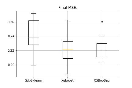
The picture will be as follows:

XGBoost has the lowest error, but XGBooBag has a more crowded error, which is definitely better: the algorithm is more stable.

That's all. I really hope that the material presented in two articles was useful, and you were able to learn something new for yourself. I am especially grateful to Dmitry for the comprehensive feedback and source codes, to Anton for the advice, to Vladimir for the difficult tasks of study.

Successes to all!

Tags: