Linear representation of the octree using the Morton code
An octave tree is a tree-like data structure, each node of which has eight descendants. Octo-trees are used for spatial indexing, collision detection in three-dimensional space, determining hidden surfaces, in ray tracing and the finite element method.
An octree can be represented as a hierarchical data structure or linearly.
In the hierarchical data structure there is a tree root, nodes and leaves. Each node stores pointers to its descendants.
With a linear representation, pointers are not used - various methods of coding elements are used and only leaves of the tree are stored.
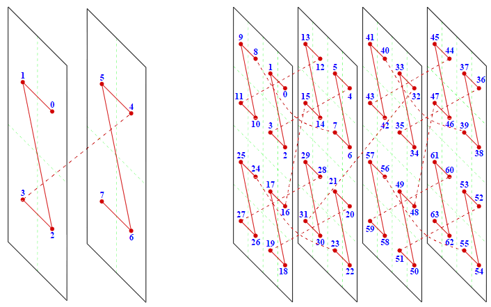
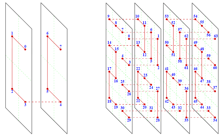
One of the most common and effective coding methods is the use of the Lebesgue curve (Z-curve) and the use of the Hilbert curve.
The advantage of the Hilbert curve is its continuity - neighboring elements are arranged in series. The advantage of the Z-curve is the simplicity and speed of calculation, so it is more often used in practice.

Two-dimensional Lebesgue curve

Three-dimensional Lebesgue curve

Two-dimensional Hilbert curve

Three-dimensional Hilbert curve
To code elements using the Z-curve, the Morton code is used (usually the code is calculated for a node with minimal coordinates). The Morton code for the Z-curve is calculated by shifting and mixing the bits of the binary representation of each coordinate.

Morton Code Calculation Example
Given the properties of the Z-curve, for elements it is necessary to store only the depth of the element (level in the octree tree) and its order (location on the Z-curve). The values of the element depth are entered into the elements of the used array for storing grid cells, and the element index determines its location on the Z-curve.
To store the depth of an element, it is enough to use 1 byte (tree depth 256). For many tasks, a tree depth of 16 may be sufficient (the size of the minimum cell will be 2 ^ 15 = 32768 times smaller than the original area). Then for storage of a cell it is enough to use 4 bits.
To determine the real coordinates of an element, the following steps must be performed:
1. calculation of the Morton code for the element
2. decoding
3. Translation of the resulting index into the real value of each coordinate.
Consider the algorithm using the example of encoding each coordinate with 20 bits, that is, the resulting code of all three coordinates will occupy 60 bits.
Knowing the code and depth of the previous element, you can calculate the code of the current element. The code of the first element is always 0. Determine the offset for each depth level:
Now we will determine the index of the element through the depth and index of the previous element:
Decoding Function:
iXYZ [0], iXYZ [1], iXYZ [2] - determine the encoding order (in this case, first the x coordinate, then y, then z).
The constants and the number of steps in the decodeIndex function are determined by the number of bits and the dimension of the space (in this example, the constants are given for three-dimensional space and 20 bits per coordinate).
There are various coding methods, examples on
Bit Twiddling Hacks
How to compute a 3D Morton number (interleave the bits of 3 ints)
To obtain real cell vertex values with minimal coordinates, the resulting indices are multiplied by the step size. The step size is the size of the minimum allowable grid cell.
The cell size can be determined by its depth. The remaining values are determined by adding the size of the elements to the corresponding minimum coordinates.
The division of the element is carried out by increasing its depth and inserting after it 7 elements of the same depth.
Merge - decrease the depth and remove the next 7 elements.
The Oktoderevo is an actively studied data structure and the algorithms for working with it (search for neighbors, intervals, visualization, etc.) become the subject of doctoral dissertations and scientific research.
An octree can be represented as a hierarchical data structure or linearly.
In the hierarchical data structure there is a tree root, nodes and leaves. Each node stores pointers to its descendants.
With a linear representation, pointers are not used - various methods of coding elements are used and only leaves of the tree are stored.
One of the most common and effective coding methods is the use of the Lebesgue curve (Z-curve) and the use of the Hilbert curve.
The advantage of the Hilbert curve is its continuity - neighboring elements are arranged in series. The advantage of the Z-curve is the simplicity and speed of calculation, so it is more often used in practice.

Two-dimensional Lebesgue curve

Three-dimensional Lebesgue curve

Two-dimensional Hilbert curve

Three-dimensional Hilbert curve
To code elements using the Z-curve, the Morton code is used (usually the code is calculated for a node with minimal coordinates). The Morton code for the Z-curve is calculated by shifting and mixing the bits of the binary representation of each coordinate.

Morton Code Calculation Example
Given the properties of the Z-curve, for elements it is necessary to store only the depth of the element (level in the octree tree) and its order (location on the Z-curve). The values of the element depth are entered into the elements of the used array for storing grid cells, and the element index determines its location on the Z-curve.
To store the depth of an element, it is enough to use 1 byte (tree depth 256). For many tasks, a tree depth of 16 may be sufficient (the size of the minimum cell will be 2 ^ 15 = 32768 times smaller than the original area). Then for storage of a cell it is enough to use 4 bits.
To determine the real coordinates of an element, the following steps must be performed:
1. calculation of the Morton code for the element
2. decoding
3. Translation of the resulting index into the real value of each coordinate.
Consider the algorithm using the example of encoding each coordinate with 20 bits, that is, the resulting code of all three coordinates will occupy 60 bits.
Knowing the code and depth of the previous element, you can calculate the code of the current element. The code of the first element is always 0. Determine the offset for each depth level:
for ( unsigned char i = 0; i < 21; ++i ) {
  levelOffset[20 - i] = offset;
  offset *= 8;
}
Now we will determine the index of the element through the depth and index of the previous element:
unsigned long getElementIndex( const unsigned long prevIndex, const unsigned char prevLevel ) {
  return prevIndex + levelOffset[prevLevel];
}
Decoding Function:
void decodeIndexXYZ( const unsigned long index, unsigned long iXYZ[3]) {
  iXYZ[0] = decodeIndex( index );
  iXYZ[1] = decodeIndex( index >> 1 );
  iXYZ[2] = decodeIndex( index >> 2 );
}
unsigned long decodeIndex( const unsigned long index ) {
  unsigned long ind = index & 0x0249249249249249;
  ind = ( ind | ( ind >> 2 ) ) & 0x00C9219243248649;
  ind = ( ind | ( ind >> 2 ) ) & 0x00386070C0E181C3;
  ind = ( ind | ( ind >> 4 ) ) & 0x0003E007C00F801F;
  ind = ( ind | ( ind >> 10 ) ) & 0x000000FFC00003FF;
  ind = ( ind | ( ind >> 20 ) ) & 0x00000000000FFFFF;
  return ind;
}
iXYZ [0], iXYZ [1], iXYZ [2] - determine the encoding order (in this case, first the x coordinate, then y, then z).
The constants and the number of steps in the decodeIndex function are determined by the number of bits and the dimension of the space (in this example, the constants are given for three-dimensional space and 20 bits per coordinate).
There are various coding methods, examples on
Bit Twiddling Hacks
How to compute a 3D Morton number (interleave the bits of 3 ints)
To obtain real cell vertex values with minimal coordinates, the resulting indices are multiplied by the step size. The step size is the size of the minimum allowable grid cell.
The cell size can be determined by its depth. The remaining values are determined by adding the size of the elements to the corresponding minimum coordinates.
The division of the element is carried out by increasing its depth and inserting after it 7 elements of the same depth.
Merge - decrease the depth and remove the next 7 elements.
The Oktoderevo is an actively studied data structure and the algorithms for working with it (search for neighbors, intervals, visualization, etc.) become the subject of doctoral dissertations and scientific research.
