Active appearance models
- From the sandbox
- Tutorial
Active Appearance Models (AAM) are statistical models of images that can be adapted to a real image through various deformations. This type of model in a two-dimensional version was proposed by Tim Kouts and Chris Taylor in 1998 [1]. Initially, active appearance models were used to estimate the parameters of facial images, but then they began to be actively applied in other areas, in particular in medicine, in the analysis of X-ray images and images obtained using magnetic resonance imaging.
This article discusses a brief description of how the active appearance models and the associated mathematical apparatus function, and provides an example of their implementation.
Over the past years, the mathematical apparatus of active appearance models has been actively developed and at the moment 2 approaches to constructing similar models can be distinguished: classic (the one that was proposed by Kutes initially) and based on the so-called inverse composition (proposed by Matthews and Baker in 2003 [2]).
We first consider the general parts of the two approaches. In active appearance models, two types of parameters are modeled: parameters associated with the shape (shape parameters), and parameters associated with the statistical image model or texture(appearance options). Before use, the model must be trained on a set of pre-marked images. The markup of images is done manually or in a semi-automatic mode, when using an algorithm there are approximate locations of labels, and then they are specified by an expert. Each label has its own number and defines a characteristic point that the model will have to find during adaptation to a new image. An example of such markup (XM2VTS face database) is shown in the figure below.
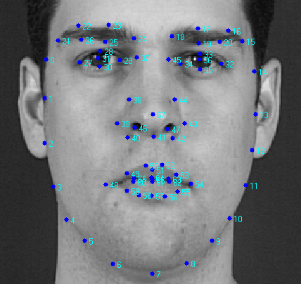
In the presented example, 68 marks are marked on the image, forming the shape of the model of the active appearance. This form denotes the external contour of the face, the contours of the mouth, eyes, nose, eyebrows. This character of the markup allows you to further determine the various parameters of the face from its image, which can be used for further processing by other algorithms. For example, it can be personal identification algorithms, audio-visual speech recognition, determining the emotional state of a subject.
The training procedure for active appearance models begins with the normalization of the position of all forms in order to compensate for differences in scale, slope and displacement. For this, the so-called generalized Prokrustov analysis is used. We will not provide a detailed description here, and an interested reader can read the corresponding Wikipedia article. This is how a lot of labels look like before and after normalization (according to [3]).
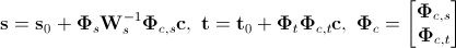
After all forms are normalized, a matrix is formed from the constituent points , where
  . After separation of the main component of said matrix we obtain the following expression for the synthesized form:
 .
.
Here is the form averaged over all implementations of the training sample (basic form),
 - matrix of principal vectors;
  - shape parameters. The above expression means that the form
  can be expressed as the sum of the basic form and a linear combination of the eigenforms contained in the matrix . By changing the vector of parameters, we can get various kinds of shape deformations to fit it to a real image. An example of such a form is shown below [7]. Blue and red arrows indicate the directions of the main components.

It should be noted that there are models of active appearance with hard and not hard deformation. Models with rigid deformation can only undergo affine transformations (rotation, shift, scaling), while models with non-rigid deformation can undergo other types of deformations. In practice, a combination of both types of deformations is used. In this case, the location parameters (rotation angle, scale, displacement or affine transformation coefficients) are also added to the shape parameters.
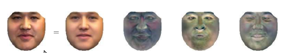
The training procedure for the components of the appearance is performed after the components of the form (basic form and matrix of principal components) are calculated. The learning process here consists of three steps. The first step is to extract textures from training images that best fit the base shape. To do this, triangulation of the marks of the basic form and the form consisting of the marks of the training image is performed. Then, using piecewise interpolation, a mapping of the regions of the training image obtained as a result of triangulation to the corresponding regions of the generated texture is performed. As an example, the figure below shows the result of such a conversion for one of the IMM database images.
After all the textures are formed, the second step is their photometric normalization in order to compensate for various lighting conditions. A large number of methods have been developed to do this. The simplest of them is subtracting the average value and normalizing the variance of pixel brightness.
Finally, in the third step, a matrix is formed from the textures, such that each of its columns contains the pixel values of the corresponding texture (similar to the matrix ) It is worth noting that the textures used for training can be either single-channel (grayscale) or multi-channel (for example, RGB color space or another). In the case of multi-channel textures, pixel vectors are formed separately for each channel, and then their concatenation is performed. After finding the principal components of the matrix texture we obtain an expression for the synthesized texture:
 .
.
Here is the basic texture obtained by averaging over all the textures of the training set,
  is the matrix of its own textures,
  is the vector of parameters of the active appearance. The following is an example of a synthesized texture [7].
In practice, to reduce the effect of retraining the model, only 95-98% of the most significant vectors are left in the matrices of the main components. Moreover, this number may be different for the main components of the form and the main components of the appearance. Refined figures can be selected already in the process of experimental studies or when testing a model using the cross-validation procedure.
On this, the general part of different types of active appearance models ends and now we will consider the differences between the two approaches.
In this type of model we must also calculate the combined vector parameter, which is defined by the following formula:
 .
.
Here is the diagonal matrix of weight values, which allows you to balance the contribution of distances between pixels and pixel intensities. For each element of the training sample (texture-form pair), its own vector is calculated
  . Then the resulting set of vectors is combined into a matrix and its main components are found. In this case, a synthesized vector of the combined shape parameters and texture is determined by the expression
 .
.
Here is the matrix of the main components of the combined parameters,
 - vector of combined appearance parameters. From here we can get a new expression for the synthesized form and texture:
 .
.
In practice, the matrix isalso subjected to the removal of noise components to reduce the effect of retraining and reduce the number of calculations.
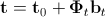
Once the parameters are calculated form, appearance and combination options, we need to find the so-called prediction matrix , which in the sense of the minimum mean square error to satisfy the following linear equation:
 .
.
Here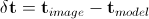 as well
 - disturbance of the position vector and combined appearance parameters. Various methods have been developed to solve the above equation. Their detailed consideration was carried out in [3 - 6].
The adaptation of the considered active appearance model to the analyzed image occurs, in the general case, as follows.
Various modifications and improvements to this algorithm have been proposed, but its general structure and essence remain the same.
The above algorithm is quite effective, but it has a rather serious drawback that limits its application in real-time applications: it converges slowly and requires a lot of computation. To overcome these shortcomings, a new type of active appearance models was proposed in [2, 7], which will be discussed in the next section.
Matthews and Baker proposed a computationally efficient algorithm for adapting an active appearance model that depends only on form parameters (the so-called “project-out” model). Due to this, it was possible to significantly increase its speed. The adaptation algorithm, which was based on the Lucas-Canada approach, uses the Newton method to find the minimum of the error function.
The Lucas-Canada algorithm tries to find the locally best match in the sense of a minimum mean square error between the template and the real image. In this case, the template is subjected to deformation (affine and / or piecewise) specified by the vector of parameters , which maps its pixels to the pixels of the real image.
Finding parameters directlyis a nonlinear optimization problem. To solve it by linear methods, the Lucas-Canada algorithm assumes that the initial value of the deformation parameters is known and then iteratively finds the increment of the parameters , updating the vector at each iteration .
The active model of the appearance of the reverse composition uses a similar approach to update its own parameters during the adaptation process, except that theanalyzed image is not subjected to deformation by the basic texture .
At the stage of training the active model of the appearance of the inverse composition, the so-called images of steepest descent and their Hessians are calculated. The adaptation of the model occurs in a manner similar to the classical model of the appearance, except that in this case only the shape parameters and (optionally) the location parameters are updated.
It is worth noting that Matthews and Baker have proposed a large number of possible variations that have different properties of the models they developed. An interested reader can refer to [2, 7 - 9] for a more detailed review.
For practical implementation and research of the above training and adaptation algorithms for active appearance models, the author has developed a specialized software library called AAMToolbox. The library is distributed under the GPLv3 license and is intended for use exclusively for non-commercial and research purposes. Source codes are available at this link .
AAMToolbox build requires OpenCV 2.4, boost 1.42 or higher libraries, NetBeans IDE 6.9. Ubuntu Linux OS versions 10.04 and 10.10 are currently supported. Performance and collection on other platforms has not been tested.
AAMToolbox implements algorithms for working with both the classic active appearance model and the active appearance model of the reverse composition. Access to both types of algorithms is through a single interface, which provides training of the model on a given training set, saving and restoring from the file of the trained model, adaptation of the model to a real image. Both color images (in three-channel color) and grayscale images are supported.
In order to train the model, you must first prepare a training sample. The selection should consist of two types of files. The first type is the actual images by which the model will be trained. Files of the second type are markup text files and contain form labels marked on the corresponding images of the training sample. The following is a fragment of such a file.
Here the first column is the label number, the second column is the X-coordinate of the label, the third column is the Y-coordinate of the label. Each image must have its own markup file.
The training code for the active appearance model is pretty simple.
As a result of the execution of the presented code fragment, it allows you to train the active model of the appearance of a given type and save it to a file. It is worth noting that during training, all data, including images, is in RAM, so when loading a large number of images (several hundred), you should make sure that a sufficient amount of it is available (2 - 3 GB). As an example of the code that conducts the training procedure for different types of active appearance models, you can see the unit test “AAM Estimator test” of the library project. If it is launched, it will train and save the models of each of the supported types in the version for color images and grayscale (in total 4 different models) into the appropriate files.
The adaptation code of the active appearance model to the image will look like this:
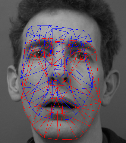
In order to see a demonstration of the adaptation algorithms for active appearance models, you need to run the unit tests “Aply model test” and “Aply model IC test”, which carry out adaptation to the image of models of supported types. The figure below shows an example of one of the results.
These tests clearly demonstrate the difference in the convergence rate of the classic active appearance model and the active appearance model of the inverse composition. However, the divergence of the latter can be attributed to the divergence of the algorithm for its adaptation in some cases. Several approaches have been proposed for its elimination, but they are not implemented in the AAMToolbox library under consideration (at least for the moment).
The article briefly examined active appearance models and related basic concepts and mathematical apparatus. AAMToolbox software library developed by the author that implements the algorithms described in the article is also considered. Examples of its use are given.
Behind the scenes were three-dimensional models of active appearance and related algorithms. Perhaps they will be discussed in the following articles.
Description of illustration
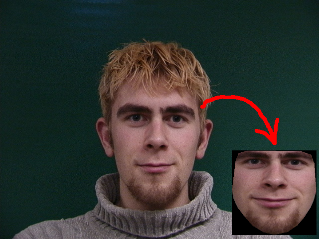
The figure shows the result of adapting the active appearance model to the face image. The blue grid shows the initial state of the model, and the red one shows what happened.
This article discusses a brief description of how the active appearance models and the associated mathematical apparatus function, and provides an example of their implementation.
Overview of Active Appearance Models
Over the past years, the mathematical apparatus of active appearance models has been actively developed and at the moment 2 approaches to constructing similar models can be distinguished: classic (the one that was proposed by Kutes initially) and based on the so-called inverse composition (proposed by Matthews and Baker in 2003 [2]).
We first consider the general parts of the two approaches. In active appearance models, two types of parameters are modeled: parameters associated with the shape (shape parameters), and parameters associated with the statistical image model or texture(appearance options). Before use, the model must be trained on a set of pre-marked images. The markup of images is done manually or in a semi-automatic mode, when using an algorithm there are approximate locations of labels, and then they are specified by an expert. Each label has its own number and defines a characteristic point that the model will have to find during adaptation to a new image. An example of such markup (XM2VTS face database) is shown in the figure below.
In the presented example, 68 marks are marked on the image, forming the shape of the model of the active appearance. This form denotes the external contour of the face, the contours of the mouth, eyes, nose, eyebrows. This character of the markup allows you to further determine the various parameters of the face from its image, which can be used for further processing by other algorithms. For example, it can be personal identification algorithms, audio-visual speech recognition, determining the emotional state of a subject.
The training procedure for active appearance models begins with the normalization of the position of all forms in order to compensate for differences in scale, slope and displacement. For this, the so-called generalized Prokrustov analysis is used. We will not provide a detailed description here, and an interested reader can read the corresponding Wikipedia article. This is how a lot of labels look like before and after normalization (according to [3]).
After all forms are normalized, a matrix is formed from the constituent points
, where . After separation of the main component of said matrix we obtain the following expression for the synthesized form: . Here
is the form averaged over all implementations of the training sample (basic form),- matrix of principal vectors; - shape parameters. The above expression means that the form can be expressed as the sum of the basic form and a linear combination of the eigenforms contained in the matrix . By changing the vector of parameters, we can get various kinds of shape deformations to fit it to a real image. An example of such a form is shown below [7]. Blue and red arrows indicate the directions of the main components.It should be noted that there are models of active appearance with hard and not hard deformation. Models with rigid deformation can only undergo affine transformations (rotation, shift, scaling), while models with non-rigid deformation can undergo other types of deformations. In practice, a combination of both types of deformations is used. In this case, the location parameters (rotation angle, scale, displacement or affine transformation coefficients) are also added to the shape parameters.
The training procedure for the components of the appearance is performed after the components of the form (basic form and matrix of principal components) are calculated. The learning process here consists of three steps. The first step is to extract textures from training images that best fit the base shape. To do this, triangulation of the marks of the basic form and the form consisting of the marks of the training image is performed. Then, using piecewise interpolation, a mapping of the regions of the training image obtained as a result of triangulation to the corresponding regions of the generated texture is performed. As an example, the figure below shows the result of such a conversion for one of the IMM database images.
After all the textures are formed, the second step is their photometric normalization in order to compensate for various lighting conditions. A large number of methods have been developed to do this. The simplest of them is subtracting the average value and normalizing the variance of pixel brightness.
Finally, in the third step, a matrix is formed from the textures, such that each of its columns contains the pixel values of the corresponding texture (similar to the matrix
) It is worth noting that the textures used for training can be either single-channel (grayscale) or multi-channel (for example, RGB color space or another). In the case of multi-channel textures, pixel vectors are formed separately for each channel, and then their concatenation is performed. After finding the principal components of the matrix texture we obtain an expression for the synthesized texture: . Here
is the basic texture obtained by averaging over all the textures of the training set, is the matrix of its own textures, is the vector of parameters of the active appearance. The following is an example of a synthesized texture [7].In practice, to reduce the effect of retraining the model, only 95-98% of the most significant vectors are left in the matrices of the main components. Moreover, this number may be different for the main components of the form and the main components of the appearance. Refined figures can be selected already in the process of experimental studies or when testing a model using the cross-validation procedure.
On this, the general part of different types of active appearance models ends and now we will consider the differences between the two approaches.
Classic Active Appearance Model
In this type of model we must also calculate the combined vector parameter, which is defined by the following formula:
. Here
is the diagonal matrix of weight values, which allows you to balance the contribution of distances between pixels and pixel intensities. For each element of the training sample (texture-form pair), its own vector is calculated . Then the resulting set of vectors is combined into a matrix and its main components are found. In this case, a synthesized vector of the combined shape parameters and texture is determined by the expression . Here
is the matrix of the main components of the combined parameters,- vector of combined appearance parameters. From here we can get a new expression for the synthesized form and texture: . In practice, the matrix is
also subjected to the removal of noise components to reduce the effect of retraining and reduce the number of calculations. Once the parameters are calculated form, appearance and combination options, we need to find the so-called prediction matrix
, which in the sense of the minimum mean square error to satisfy the following linear equation: . Here
as well- disturbance of the position vector and combined appearance parameters. Various methods have been developed to solve the above equation. Their detailed consideration was carried out in [3 - 6]. The adaptation of the considered active appearance model to the analyzed image occurs, in the general case, as follows.
- Based on the initial approximation, all model parameters and affine form transformations are calculated;
- The error vector is calculated
 . Extracting the texture from the analyzed image occurs using its piecewise deformation;
 - The vector of perturbations is calculated ;
- The vector of combined parameters and affine transformations is updated by summing their current values with the corresponding components of the perturbation vector;
- The shape and texture are being updated;
- We proceed to fulfillment of point 2 until we reach convergence.
Various modifications and improvements to this algorithm have been proposed, but its general structure and essence remain the same.
The above algorithm is quite effective, but it has a rather serious drawback that limits its application in real-time applications: it converges slowly and requires a lot of computation. To overcome these shortcomings, a new type of active appearance models was proposed in [2, 7], which will be discussed in the next section.
Active model of the appearance of the reverse composition
Matthews and Baker proposed a computationally efficient algorithm for adapting an active appearance model that depends only on form parameters (the so-called “project-out” model). Due to this, it was possible to significantly increase its speed. The adaptation algorithm, which was based on the Lucas-Canada approach, uses the Newton method to find the minimum of the error function.
The Lucas-Canada algorithm tries to find the locally best match in the sense of a minimum mean square error between the template and the real image. In this case, the template is subjected to deformation (affine and / or piecewise) specified by the vector of parameters
, which maps its pixels to the pixels of the real image. Finding parameters directly
is a nonlinear optimization problem. To solve it by linear methods, the Lucas-Canada algorithm assumes that the initial value of the deformation parameters is known and then iteratively finds the increment of the parameters , updating the vector at each iteration . The active model of the appearance of the reverse composition uses a similar approach to update its own parameters during the adaptation process, except that the
analyzed image is not subjected to deformation by the basic texture .At the stage of training the active model of the appearance of the inverse composition, the so-called images of steepest descent and their Hessians are calculated. The adaptation of the model occurs in a manner similar to the classical model of the appearance, except that in this case only the shape parameters and (optionally) the location parameters are updated.
It is worth noting that Matthews and Baker have proposed a large number of possible variations that have different properties of the models they developed. An interested reader can refer to [2, 7 - 9] for a more detailed review.
Software implementation
For practical implementation and research of the above training and adaptation algorithms for active appearance models, the author has developed a specialized software library called AAMToolbox. The library is distributed under the GPLv3 license and is intended for use exclusively for non-commercial and research purposes. Source codes are available at this link .
AAMToolbox build requires OpenCV 2.4, boost 1.42 or higher libraries, NetBeans IDE 6.9. Ubuntu Linux OS versions 10.04 and 10.10 are currently supported. Performance and collection on other platforms has not been tested.
AAMToolbox implements algorithms for working with both the classic active appearance model and the active appearance model of the reverse composition. Access to both types of algorithms is through a single interface, which provides training of the model on a given training set, saving and restoring from the file of the trained model, adaptation of the model to a real image. Both color images (in three-channel color) and grayscale images are supported.
In order to train the model, you must first prepare a training sample. The selection should consist of two types of files. The first type is the actual images by which the model will be trained. Files of the second type are markup text files and contain form labels marked on the corresponding images of the training sample. The following is a fragment of such a file.
1 228 307
2 232 327
3 239 350
5 270 392
6 294 406
7 314 410
8 343 403
9 361 388
10 372 370
11 382 349
12 388 331
13 393 312
14 374 243
Here the first column is the label number, the second column is the X-coordinate of the label, the third column is the Y-coordinate of the label. Each image must have its own markup file.
The training code for the active appearance model is pretty simple.
#include "aam/AAMEstimator.h"
void trainAAM()
{
    // Создаем объект оценивателя параметров модели
    aam::AAMEstimator estimator;
    // Здесь будет хранится список файлов, которые
    // составят обучающую выборку
    // aam::ModelPathType является алиасом для пары
    // std::pair, первый компонент
    // которой должен содержать путь к файлу меток, а
    // второй - путь к обучающему изображению.
    std::vector modelPaths;
    // Заполняем каким-либо образом наш список файлов
    ......................................................
    //
    // Теперь устанавливаем параметры обучения в опциях
    aam::TrainOptions options;
    // Порог отсечения шумовых главных компонент. Принимает значения от 0 до 1.
    options.setPCACutThreshold(0.95);
    // Выбираем, по каким изображениям производить обучение:
    // true - градации серого, false - цветные трехканальные
    options.setGrayScale(true);
    // Проводить ли обучение в несколько параллельных потоков.
    // Актуально при выборе классической активной модели
    // внешнего вида.
    options.setMultithreading(true);
    // Выбираем алгоритм обучения модели:
    // aam::algorithm::conventional - классическая модель,
    // aam::algorithm::inverseComposition - модель обратной композиции
    options.setAAMAlgorithm(aam::algorithm::conventional);
    // Устанавливаем результат триангуляции. Необходимо не во всех случаях.
    // Если не устанавливать, то в процессе обучения триангуляция будет
    // проведена автоматически. В противном случае переменная triangles должна
    // иметь тип std::vector и содержать список номеров вершин
    // треугольников (нумерация вершин начинается с 0.
    options.setTriangles(triangles);
    // Устанавливаем количество уровней гауссовой пирамиды изображений.
    // Ее использование предполагает обучение модели на нескольких масштабах,
    // что позволяет снизить риск попадания в локальный минимум.
    options.setScales(4);
    estimator.setTrainOptions(options);
    // Собственно процедура обучения
    estimator.train(modelPaths);
    // Сохраняем обученную модель в файл
    estimator.save("data/aam_test.xml");
}
As a result of the execution of the presented code fragment, it allows you to train the active model of the appearance of a given type and save it to a file. It is worth noting that during training, all data, including images, is in RAM, so when loading a large number of images (several hundred), you should make sure that a sufficient amount of it is available (2 - 3 GB). As an example of the code that conducts the training procedure for different types of active appearance models, you can see the unit test “AAM Estimator test” of the library project. If it is launched, it will train and save the models of each of the supported types in the version for color images and grayscale (in total 4 different models) into the appropriate files.
The adaptation code of the active appearance model to the image will look like this:
#include "aam/AAMEstimator.h"
void aplyAAM()
{
    // Загружаем модель.
    // Ее тип и алгоритм работы будет определен автоматически
    aam::AAMEstimator estimator;
    estimator.load("<путь_к_файлу_модели>");
    // Загружаем картинку
    cv::Mat im = cv::imread("<путь_к_файлу_изображения>");
    // Определяем положение лица на изображении
    std::vector faces;
    cv::cvtColor(im, im, CV_BGR2GRAY);
    cascadeFace.detectMultiScale(im, faces,
            1.1, 2, 0
            |CV_HAAR_FIND_BIGGEST_OBJECT
            //|CV_HAAR_DO_ROUGH_SEARCH
            |CV_HAAR_SCALE_IMAGE
            ,
            cv::Size(30, 30) );
    if (faces.empty())
    {
        return;
    }
    cv::Rect r = faces[0];
    aam::Point2D startPoint(r.x + r.width * 0.5 + 20, r.y +
            r.height * 0.5 + 40);
    // Массив, куда будут помещены координаты точек найденной формы
    aam::Vertices2DList foundPoints;
    // Производим адаптацию модели. Последний параметр verbose определяет
    // выводить диагностическую информацию процесса адаптации или нет.
    estimator.estimateAAM(im, startPoint, foundPoints, true);
}
In order to see a demonstration of the adaptation algorithms for active appearance models, you need to run the unit tests “Aply model test” and “Aply model IC test”, which carry out adaptation to the image of models of supported types. The figure below shows an example of one of the results.
These tests clearly demonstrate the difference in the convergence rate of the classic active appearance model and the active appearance model of the inverse composition. However, the divergence of the latter can be attributed to the divergence of the algorithm for its adaptation in some cases. Several approaches have been proposed for its elimination, but they are not implemented in the AAMToolbox library under consideration (at least for the moment).
Conclusion
The article briefly examined active appearance models and related basic concepts and mathematical apparatus. AAMToolbox software library developed by the author that implements the algorithms described in the article is also considered. Examples of its use are given.
Behind the scenes were three-dimensional models of active appearance and related algorithms. Perhaps they will be discussed in the following articles.
List of references
- T. Cootes, G. Edwards, and C. Taylor. Active appearance models. In Proceedings of the European Conference on Computer Vision, volume 2, pages 484–498, 1998.
- S. Baker, R. Gross, and I. Matthews. Lucas-Kanade 20 years on: A unifying framework: Part 3. Technical Report CMU-RI-TR-03-35, Carnegie Mellon University Robotics Institute, 2003.
- MB Stegmann Analysis and Segmentation of Face Images using Point Annotations and Linear Subspace Techniques. Technical report IMM-REP-2002-22-22, Informatics and Mathematical Modeling, Technical University of Denmark, 2002
- TF Cootes, GJ Edwards, and CJ Taylor. Active appearance models. IEEE Trans. on Pattern Recognition and Machine Intelligence, 23 (6): 681–685, 2001.
- TF Cootes and CJ Taylor. Statistical models of appearance for medical image analysis and computer vision. In Proc. SPIE Medical Imaging 2001, volume 1, pages 236–248. SPIE, 2001.
- TF Cootes and CJ Taylor. Constrained active appearance models. Computer Vision, 2001. ICCV 2001. Proceedings. Eighth IEEE International Conference on, 1: 748–754 vol. 1, 2001.
- Iain Matthews and Simon Baker Active Appearance Models Revisited. International Journal of Computer Vision, Vol. 60, No. 2, November, 2004, pp. 135 - 164.
- S. Baker, R. Gross, and I. Matthews. Lucas-Kanade 20 years on: A unifying framework: Part 1. Technical Report CMU-RI-TR-02-16, Carnegie Mellon University Robotics Institute, 2002.
- S. Baker, R. Gross, and I. Matthews. Lucas-Kanade 20 years on: A unifying framework: Part 2. Technical Report CMU-RI-TR-03-01, Carnegie Mellon University Robotics Institute, 2003.