Autoencoders and Strong AI
The theory of autoencoders and generating models has recently received serious development, but quite a few works have been devoted to how to use them in recognition problems. At the same time, the property of autoencoders to obtain a hidden parametric data model and mathematical consequences of this make it possible to associate them with Bayesian decision-making methods.
The article proposes an original mathematical apparatus “a set of auto-encoders with a common latent space”, which allows you to select abstract concepts from the input data and demonstrates the ability to “one-shot learning”. In addition, it can overcome many of the fundamental problems of modern machine learning algorithms based on multilayer networks and the “Deep learning” approach.
Artificial neural networks, which are trained using the mechanism of back-propagation of errors, practically crowded out other approaches in many problems of recognition and parameter estimation. But they have a number of shortcomings that seem to be fixable without a serious review of the approach:
Being engaged in the solution of applied problems, and, relying on a number of existing works, I propose an approach that differs markedly from the existing ones, eliminates a number of their shortcomings and is applicable for solving applied problems in various fields of machine learning.
In decision theory, a very important place is occupied by the density of distribution (or distribution function) of random variables. It is necessary to have estimates of the distribution functions for the calculation of a posteriori risk.
It turns out that autoencoders are very natural to perform the evaluation of distribution functions. This can be explained as follows: the training data set is determined by the density of their distribution. The higher the density of teaching examples around a local point in the input space, the better the autoencoder will reconstruct the input vector in this place of space. In addition, inside the autoencoder there is a vector of latent representation of the input data (usually of low dimensionality), and if the data is projected in the latent space into an area not previously involved in the training, then there is nothing similar in the training set.
There are a number of closed and in some separate works:
The first is the rationale that the result of Denoising autoencoder reconstruction is related to the probability density function of the input data, but a number of restrictions are imposed on the autoencoders. In the second, sufficient requirements for the autoencoder are given - the weights of the encoder and decoder must be “connected”, i.e. The weight matrix of the encoder layer is the transpose matrix of the decoder. In the last work, the necessary and sufficient conditions for the fact that the auto-encoder is related to the probability density are more fully investigated.
These works strictly substantiate the theoretical basis for the connection of autoencoders with the distribution density of training data. In applied problems, such a serious analysis is often not required; therefore, a slightly different approach will be given below, which makes it possible to evaluate the probability density function of input data at the expense of a previously trained autoencoder.
In even earlier works, an empirical idea was proposed that for the task of classification, autoencoders could be trained in the number of classes (teaching each of them only on a subsample corresponding to it). And choose the class and autoencoder that gives the minimum discrepancy between the input image and the reconstructed one. It was not difficult to check on MNIST: train 10 autoencoders (for each digit), calculate the accuracy, and then compare it with a similar multilayer classifier model.
Scripts for training and testing on git (train_ae.py, calc_codes.py, calc_acc.py)
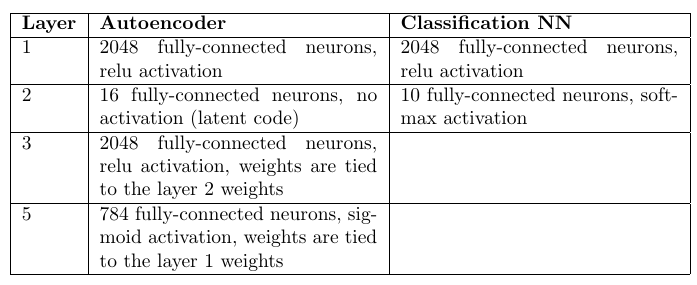
Architecture and number of scales:
Autoencoders: 98.6%
Classifier on a multilayer perceptron: 98.4%
An attentive reader will notice that there were 10 times more weights in autoencoders (by their number). However, a 10-fold increase in the number of scales in a hidden layer in a multilayer perceptron only worsens the statistics.
Of course, convolutional networks provide much higher accuracy, but the task was only to compare the approaches with other things being equal.
As a result, it can be noted that the approach with autoencoders is quite competitive with fully connected networks. And, although the time required to optimize the scales is much more, it has one important advantage: the ability to detect anomalies in the input data. If none of the autoencoders could accurately reconstruct the input image, then it can be stated that an anomalous image got into the input that was not encountered in the training set. Strictly speaking, you can reconstruct the image and not from the input sample, but what to do in such a situation will be shown below.
It is possible, and in a slightly different way than in the above works, to carry out a qualitative analysis of the relationship between the probability density of the input data p (x) and the auto-encoder response.
Autoencoder - sequential use of the encoder function and decoder
  where
where  - input vector, and
  - latent view. In some subset of the input data (usually close to the tutorial)
 where
where  - discrepancy. The discrepancy will be accepted by Gaussian noise (its parameters can be estimated after learning of the auto-encoder). As a result, a number of rather strong assumptions are made:
1) discrepancy - Gaussian noise
2) the autoencoder is already “trained” and works
But, importantly, the autoencoder itself will not be superimposed with almost no restrictions.
Next, you can get a qualitative estimate of the probability density p (x), on the basis of which you can draw several very important conclusions in the future.
Distribution density for and
and  related as follows:
We need to get the connection p (x) and p (z). For some autoencoders, p (z) is set at the training stage, for others p (z), it is still easier to obtain due to the smaller dimensionality Z.
The distribution density of the residual n is known, which means:
 Is the distance between x and its projection x *. At some point z *, this distance will reach its minimum. At this point, the partial derivatives of the argument of the exponent in formula (2) with respect to
 (Z-axis) will be zero:
Here scalar, then:
The choice of the point z *, where the distanceminimal, due to the process of optimizing the auto-encoder. During training, it is the quadratic discrepancy that is minimized (as a rule): where
where  - autoencoder weight. Those. after learning g (x) tends to z *.
We can also decompose in taylor series (before the first term) around z *:
So, now equation (2) will become:
Note that the last factor is 1 due to the expression (3). The first factor can be taken out of the integral sign (it does not contain z) in (1). And also suppose that p (z) is a sufficiently smooth function and does not change much in the neighborhood of z *, i.e. replace p (z) -> p (z *).
After all the assumptions, integral (1) has the estimate:
Where
The last integral is the n-dimensional Euler-Poisson integral:
As a result, we received the final estimate of p (x):
All this mathematics was needed to show that p (x) depends on three factors:
And from the normalization constant, which will later be responsible for the a priori probability of choosing an autoencoder to describe the input data.
Despite all the assumptions, the result was very meaningful and useful from the point of view of calculations.
Now it is possible to more accurately describe the classification procedure using a set of auto-encoders:
And for each input vector you can now evaluate by the number of classes. And this will be the likelihood function, which is necessary for decision-making under the Bayesian decision rule.
In the same way, it is also possible to estimate unknown parameters by dividing the parameter space into discrete values, having trained your own autoencoder for each value. And then, based on the best Bayesian estimate, choose the value that gives the maximum likelihood function.
It is worth noting here that, formally, the task of estimating p (z) is not at all simpler than estimating p (x). But in practice it is not. The space Z usually has a much smaller dimension, or, in general, the distribution is specified when optimizing the weights of the auto-encoder.
There is a curious interpretation proposed by Alexei Redozubov and described in the following articles:
Information may have completely different interpretations in different contexts. The “autoencoder set” model echoes this proposed idea. Any autoencoder is a latent model of input data within one context (one class or other fixed parameters), i.e. latent vector - interpretation, and each autoencoder - context. When input information is received, it is considered in each context (by each autoencoder), and the context that is most likely to be chosen taking into account the existing models in each autoencoder is chosen.
The next sensible step would be to allow the existence of intersections of interpretations in various contexts. Those. when learning, we often know that the interpretation remains the same, but the form of presentation (context) changes. For example, the orientation of an object changes, but the object remains the same. The vector of the description of the object must be preserved, and the context - the orientation changes.
Then, if we look at the formula (4), then the factor p (z) can be estimated for the entire set of autoencoders, and not for each separately. The treatment (latent vector) will have a common distribution. For a small number of autoencoders, this may not be significant, but in a real task this number can be huge. For example, if you define one context for each possible orientation of a 3D object, there may be hundreds of thousands of them. Now each example presented for training in any context will form the distribution p (z).
In an applied task, the question will immediately arise: what should be assigned to interpretation, and what should be the context? Context and interpretation can be easily reversed, and no one excludes the possibility of the simultaneous parallel operation of a pair of “autoencoder sets”.
For clarity, we can offer the following example: The
input image contains people's faces.
The optimal Bayesian decision in the first case will be made regarding the orientation of the face, and in the second - its type. Presumably, the first option will give the best accuracy in orientation, and the second more accurately estimate whose face it was.
When learning, we need to know how an entity within its meaning looks in different contexts. For example, if we talk about the image of numbers and context-orientation, then this cross-learning is schematically as follows: The

encoder of one autoencoder is used, then the latent code is decoded by the decoder of another autoencoder. The learning loss function remains standard. It is interesting that if the autoencoder is selected symmetrical (i.e., the weights of the encoder and decoder are related), then in each iteration all the weights of both autoencoders are optimized.
The most convenient approach for such tricky training is PyTorch, which allows you to make quite complex back-propagation schemes for errors, including dynamic ones.
The standard learning steps of each autoencoder alternate with iterations of cross-learning. As a result, all autoencoders get a common latent space or bind “treatment” in various contexts.
It is very important that as a result of this analysis we will be able to divide the input information into “context” and “interpretation”.
Consider a fairly simple example based on MNIST, which will help demonstrate the principle of learning autoencoders with a common latent space. As a result, this example will demonstrate the formation of an abstract concept of a “cube” using the mechanism described in the article.
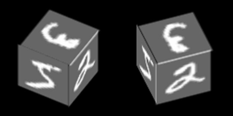
Figures from MNIST are drawn on the faces of the cube and it rotates around one of its axes:
We will teach autoencoders to restore the faces, the context is the orientation of the face.
Here is an example of the number “zero” in 100 contexts, the first 34 of which correspond to different angles of rotation of the side face, and the remaining 76 contexts - different angles of rotation of the upper face.

We assume that for each of these 100 images, the “interpretations” should be the same, and it is their random combinations that are used for cross-training.
After learning by the method described above, it was possible to achieve the fact that the latent code of one of the autoencoders can be decoded by other autoencoders, having received a really meaningful contextual transformation.
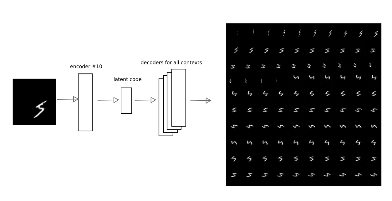
For example, this image shows how the result of coding autoencoder number 10 is decoded by other autoencoders for one of the numbers:
Thus, having the code of "interpretation", i.e. the latent vector of the autoencoder, you can restore the original image in any of the trained contexts (i.e., the decoder of any autoencoder).
In the formula (4), the variance of the residual appears everywhere , which is chosen constant for any of the components of the input vector. However, if some components do not have any statistical connection with the latent model, then the dispersion will probably be much higher for these components. Dispersion is everywhere in the denominator, and, therefore, the larger the discrepancy, the less the contribution of the error in the component. You can treat this as a masking of some part of the input vector.
For this example with rotating faces, the mask is obvious - the projection of the face in a particular context.

In the simplified approach in this example, which uses only the discrepancy between the input image and the reconstruction, you only need to multiply the residual by the mask for each of the contexts.
In general, it is necessary to more strictly evaluate the distribution parameters, thus not entering the mask manually.
By separating the interpretation from the context, you can get abstract concepts. In a trained example, it is interesting to demonstrate 2 effects:
1) one-shot learning, i.e. learning with a super small number of examples (in the limit of one).
If we analyze only the interpretation, ignoring the context, then it becomes possible to recognize a new image in different orientations of the face, when a new image was demonstrated only in one of the orientations.
It is important to note that the image must be presented new. For correctness, we will also set ourselves the goal of remembering not one image, but learning how to separate 2 new images that are not previously encountered in the MNIST training base. For example, such:

The idea is as follows: show these signs in one of the geometrical contexts (for example, number 10), choose a hyperplane that is equidistant from interpretations of these signs, and then make sure that with the help of this hyperplane we will be able to recognize that the sign was presented to us as the face rotates (other contexts).
It is important to note here that autoencoders will not learn new signs. Due to the variety of numbers that MNIST has, it is possible to predict what the new sign, which has not previously been encountered, will look like in different contexts.
So the V sign will look after encoding in the context of №10 and decoding in the remaining ones:

It can be seen that the prediction is not perfect, but visually recognizable.
We denote this demonstration “experiment 1” and describe the result below.
2) and with a cube it is interesting to demonstrate what will happen if you ignore the contents of the latent vector, and transfer only the likelihood degree of each autoencoder.
Let's see what the likelihood degree looks like for each of the contexts for two cubes with completely different textures (figures 5 and 9) for 100 contexts that can be displayed as a map: You

can see that the maps are quite similar, despite the different textures on the sides of the cube.
Those. the vector itself, which contains the plausibility of autoencoder models (contexts), allows us to formulate a new abstract concept related to the 3-dimensional cube shape. This vector can also be described at the next level by an autoencoder that learns the cube model.
In the second experiment, you will need to create a second level of information processing in which to teach the auto-encoder of the abstract cube model. And, then, using the reverse projection to restore the original image for different implementations of the model of this cube. Simply put, make the cube rotate.
A set of autoencoders trained in MNIST is applied to two new images presented in the context of # 10. There are 2 points in the latent space corresponding to the signs V and +. We define a plane equidistant from both points, which we will use to make a decision. If the point is on one side of the plane - the sign V, on the other - the plus sign.
Now we will get the codes of the transformed images and for each of them we will calculate the distance to the plane, keeping the sign.
As a result, it is possible to distinguish what kind of sign was presented for all 100 contexts.
Distribution of distances on the graph:

Visualization of the result on the example of individual characters:
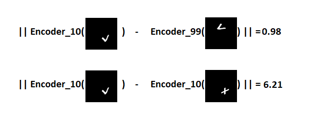
Those. latent codes of V signs in completely different contexts are much closer to each other in the latent space than codes of V and plus signs in the same context. Due to this, in 100 out of 100 cases, it is possible to successfully distinguish the signs in various orientations of the faces of the cube, despite the fact that only one sample of each sign was presented.
It was possible to demonstrate the classic "one-shot learning", which is impossible in the original architecture of artificial neural networks. The basic principle by which this approach works is very similar to “transfer learning”, demonstrated, for example, in this article .
Link to git (train_ae_shared.py, test_AB.py)
Separating the treatment from the context also allows you to study on a limited set of examples. It is possible to demonstrate only one of the possible interpretations in different contexts (fixing the "latent vector"). An abstract model of a cube can be obtained just by showing only one digit on all faces.
The experiment is constructed as follows:
The training set consisted of 5421 images with the image of the figure 5 on the sides, example:

cubes with rotation from 0 to 90 degrees
We know in advance that the cube has only one degree of freedom of rotation, therefore the autoencoder at the second level has only one component in the latent code. After learning, you can vary this component from 0 to 1 (the sigmoid was chosen to activate the latent layer) and see what the likelihood vector of contexts is reproduced during decoding:

Then this vector is transferred to level 1, in which 100 face orientation contexts, local maxima and “ any latent mark code on the faces of a cube is imagined. “Imagine” the number 3 on the edges, changing the latent vector in the autoencoder responsible for the abstract cube concept, and we obtain the following image of the cube:

Or the code of the sign V, which was not met at all in the training set:

Quality is worse, but the sign is recognizable.
Thus, at the second level of image processing, we obtained an autoencoder, which models a variety of the abstract notion “cube”. In practice, in the problems of recognition, the principle of reverse projection, shown in the experiment, is extremely important, since allows you to eliminate the ambiguities of interpretation due to the formation of abstract concepts of a higher level.
Link to git (second_level.py, second_level_test.py)
In my previous article, when recognizing license plates, a similar method was used without explanation. The position, orientation and scale of the figure in the image were separated from the content, the next level perceived this data to build a “car number” model. No matter what the numbers are, their mutual geometric configuration is important, so that we can confidently say that this is a car number (by the way, also an abstract concept).
By analogy, we can cite a number of other examples from computer vision: the 3D shape of an object or its outlines are separable from its texture and background; the enumeration of the constituent parts in isolation from the mutual spatial configuration also often allows us to form a new abstract concept.
It is also interesting how in other areas of machine learning this can work: highlighting the melody of a song is also a rejection of the interpretation (which particular vowel is pronounced) and the use of only the context (pitch height); grammatical constructions (patterning, for example, “someone did something”).
At the moment it is difficult to formulate, what is the difference between a strong AI and a weak one. Probably, this list should include all that is missing from existing approaches and algorithms for computers to act as efficiently as a person, for example:
There is also clearly a lack of developed memory mechanisms integrated with the learning process, reward / punishment mechanisms.
The article demonstrates the approach to the problem of recognition and parameter estimation, which is based on the choice of the best model that describes the input data. It is assumed that this is the mechanism for choosing the best interpretation and context. Due to the separation of interpretation and context at the output of the module (set of autoencoders), it is possible to formulate abstract concepts or to generalize experience in isolation from the context, thereby reducing the training sample. Sets of contexts can reflect the readings of the sensors of the machine (orientation, position, speed, etc.), due to which natural learning without a teacher becomes possible.
In addition, despite the fact that in learning of autoencoders, deep learning is used, the processes occurring in autoencoders are easily analyzed at each level of information processing, since it is possible to determine within which model (or in what context) the best interpretation was found. And the meaning of feedback between the levels that need to be entered in complex systems is an increase or decrease in the probability of choosing one or another context.
A mathematical apparatus is proposed, on the basis of which one can choose a particular model that describes the input data, guided by the Bayesian decision rule. Models are obtained using autoencoders with a common latent space. The idea was proposed, according to which the autoencoder's latent code is an interpretation, and the latent model, i.e. The autoencoder itself is a context.
It has been demonstrated that the set of autoencoders in itself is not inferior in accuracy to fully connected artificial neural networks using the example of MNIST.
The effect of separating the interpretation from the context is shown: minimization of the required data set (in the “one-shot learning” limit) for recognizing newly presented images due to pre-training on other data.
The effect from the separation of context from interpretation is shown: the possibility of the formation of abstract concepts of the next level on the example of the geometric abstraction "cube".
1) Alain, G. and Bengio, Y. What regularized autoencoders learn from the data generating distribution. 2013.
2) Kamyshanska, H. 2013. On autoencoder scoring
3) Im Daniel Jiwoong, Mohamed Ishmael Belghazi, Roland Memisevic. 2016. Conservativeness of Untied Auto-Encoders
4) Cortical Minicolumns. Vasily Morzhakov, Alexey Redozubov
5) Holographic Memory: Neural Microcircuits. Alexey Redozubov, Springer
6) Not at all neural networks. Morzhakov V.
7) en.wikipedia.org/wiki/Gaussian_integral
8)Adversarial Examples: Attacks and Defenses for Deep Learning
9) One-Shot Imitation Learning
PS: This article is a Russian-language electronic preprint published for discussing results, searching for errors. Any constructive criticism is welcome!
The article proposes an original mathematical apparatus “a set of auto-encoders with a common latent space”, which allows you to select abstract concepts from the input data and demonstrates the ability to “one-shot learning”. In addition, it can overcome many of the fundamental problems of modern machine learning algorithms based on multilayer networks and the “Deep learning” approach.
Prerequisites
Artificial neural networks, which are trained using the mechanism of back-propagation of errors, practically crowded out other approaches in many problems of recognition and parameter estimation. But they have a number of shortcomings that seem to be fixable without a serious review of the approach:
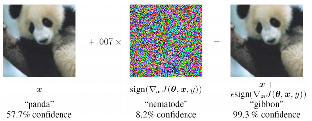
- extreme instability to input data not found in the training set (including in the case of Adversarial attacks)
- it is difficult to assess the source of the problem and locally retrain at one of the levels (you just have to supplement the training sample and retrain), i.e. black box problem
- the possibility of different interpretations of the same input information is not provided, the statistical nature of the observed data is ignored

Being engaged in the solution of applied problems, and, relying on a number of existing works, I propose an approach that differs markedly from the existing ones, eliminates a number of their shortcomings and is applicable for solving applied problems in various fields of machine learning.
Autoencoder to estimate distribution density
In decision theory, a very important place is occupied by the density of distribution (or distribution function) of random variables. It is necessary to have estimates of the distribution functions for the calculation of a posteriori risk.
It turns out that autoencoders are very natural to perform the evaluation of distribution functions. This can be explained as follows: the training data set is determined by the density of their distribution. The higher the density of teaching examples around a local point in the input space, the better the autoencoder will reconstruct the input vector in this place of space. In addition, inside the autoencoder there is a vector of latent representation of the input data (usually of low dimensionality), and if the data is projected in the latent space into an area not previously involved in the training, then there is nothing similar in the training set.
There are a number of closed and in some separate works:
- Alain, G. and Bengio, Y. What regularized autoencoders learn from the data generating distribution. 2013
- Kamyshanska, H. 2013. On autoencoder scoring
- Daniel Jiwoong Im, Mohamed Ishmael Belghazi, Roland Memisevic. 2016. Conservativeness Untied Auto-Encoders
The first is the rationale that the result of Denoising autoencoder reconstruction is related to the probability density function of the input data, but a number of restrictions are imposed on the autoencoders. In the second, sufficient requirements for the autoencoder are given - the weights of the encoder and decoder must be “connected”, i.e. The weight matrix of the encoder layer is the transpose matrix of the decoder. In the last work, the necessary and sufficient conditions for the fact that the auto-encoder is related to the probability density are more fully investigated.
These works strictly substantiate the theoretical basis for the connection of autoencoders with the distribution density of training data. In applied problems, such a serious analysis is often not required; therefore, a slightly different approach will be given below, which makes it possible to evaluate the probability density function of input data at the expense of a previously trained autoencoder.
MNIST example
In even earlier works, an empirical idea was proposed that for the task of classification, autoencoders could be trained in the number of classes (teaching each of them only on a subsample corresponding to it). And choose the class and autoencoder that gives the minimum discrepancy between the input image and the reconstructed one. It was not difficult to check on MNIST: train 10 autoencoders (for each digit), calculate the accuracy, and then compare it with a similar multilayer classifier model.
Scripts for training and testing on git (train_ae.py, calc_codes.py, calc_acc.py)
Architecture and number of scales:
Autoencoders: 98.6%
Classifier on a multilayer perceptron: 98.4%
An attentive reader will notice that there were 10 times more weights in autoencoders (by their number). However, a 10-fold increase in the number of scales in a hidden layer in a multilayer perceptron only worsens the statistics.
Of course, convolutional networks provide much higher accuracy, but the task was only to compare the approaches with other things being equal.
As a result, it can be noted that the approach with autoencoders is quite competitive with fully connected networks. And, although the time required to optimize the scales is much more, it has one important advantage: the ability to detect anomalies in the input data. If none of the autoencoders could accurately reconstruct the input image, then it can be stated that an anomalous image got into the input that was not encountered in the training set. Strictly speaking, you can reconstruct the image and not from the input sample, but what to do in such a situation will be shown below.
Consider a single autoencoder
It is possible, and in a slightly different way than in the above works, to carry out a qualitative analysis of the relationship between the probability density of the input data p (x) and the auto-encoder response.
Autoencoder - sequential use of the encoder function
and decoder where - input vector, and - latent view. In some subset of the input data (usually close to the tutorial)where - discrepancy. The discrepancy will be accepted by Gaussian noise (its parameters can be estimated after learning of the auto-encoder). As a result, a number of rather strong assumptions are made: 1) discrepancy - Gaussian noise
2) the autoencoder is already “trained” and works
But, importantly, the autoencoder itself will not be superimposed with almost no restrictions.
Next, you can get a qualitative estimate of the probability density p (x), on the basis of which you can draw several very important conclusions in the future.
P (x) rating for a single autoencoder
Distribution density for
and related as follows:
We need to get the connection p (x) and p (z). For some autoencoders, p (z) is set at the training stage, for others p (z), it is still easier to obtain due to the smaller dimensionality Z.
The distribution density of the residual n is known, which means:

Is the distance between x and its projection x *. At some point z *, this distance will reach its minimum. At this point, the partial derivatives of the argument of the exponent in formula (2) with respect to (Z-axis) will be zero:
Here
scalar, then:
The choice of the point z *, where the distance
minimal, due to the process of optimizing the auto-encoder. During training, it is the quadratic discrepancy that is minimized (as a rule):where - autoencoder weight. Those. after learning g (x) tends to z *. We can also decompose
in taylor series (before the first term) around z *:
So, now equation (2) will become:


Note that the last factor is 1 due to the expression (3). The first factor can be taken out of the integral sign (it does not contain z) in (1). And also suppose that p (z) is a sufficiently smooth function and does not change much in the neighborhood of z *, i.e. replace p (z) -> p (z *).
After all the assumptions, integral (1) has the estimate:

Where
The last integral is the n-dimensional Euler-Poisson integral:

As a result, we received the final estimate of p (x):

All this mathematics was needed to show that p (x) depends on three factors:
- The distance between the input vector and its reconstruction, the worse it was restored - the less p (x)
- Probability densities p (z *) at z * = g (x)
- Normalization of the function p (z) at the point z *, which is calculated for the auto-encoder from the partial derivatives of the function f
And from the normalization constant, which will later be responsible for the a priori probability of choosing an autoencoder to describe the input data.
Despite all the assumptions, the result was very meaningful and useful from the point of view of calculations.
The procedure for the classification or evaluation of parameters
Now it is possible to more accurately describe the classification procedure using a set of auto-encoders:
- Independent autoencoder training for each class on the relevant output
- Calculation of the matrix W for each autoencoder
- Estimate p (z) for each autoencoder
And for each input vector you can now evaluate
by the number of classes. And this will be the likelihood function, which is necessary for decision-making under the Bayesian decision rule. In the same way, it is also possible to estimate unknown parameters by dividing the parameter space into discrete values, having trained your own autoencoder for each value. And then, based on the best Bayesian estimate, choose the value that gives the maximum likelihood function.
It is worth noting here that, formally, the task of estimating p (z) is not at all simpler than estimating p (x). But in practice it is not. The space Z usually has a much smaller dimension, or, in general, the distribution is specified when optimizing the weights of the auto-encoder.
The idea of combining the latent space of autoencoders
There is a curious interpretation proposed by Alexei Redozubov and described in the following articles:
- An Artificial Neural Architecture Cortical Minicolumns. Vasily Morzhakov, Alexey Redozubov
- Holographic Memory: A model for information processing by Neural Microcircuits. Alexey Redozubov, Springer
- Not neural networks at all. Morzhakov V.
Information may have completely different interpretations in different contexts. The “autoencoder set” model echoes this proposed idea. Any autoencoder is a latent model of input data within one context (one class or other fixed parameters), i.e. latent vector - interpretation, and each autoencoder - context. When input information is received, it is considered in each context (by each autoencoder), and the context that is most likely to be chosen taking into account the existing models in each autoencoder is chosen.
The next sensible step would be to allow the existence of intersections of interpretations in various contexts. Those. when learning, we often know that the interpretation remains the same, but the form of presentation (context) changes. For example, the orientation of an object changes, but the object remains the same. The vector of the description of the object must be preserved, and the context - the orientation changes.
Then, if we look at the formula (4), then the factor p (z) can be estimated for the entire set of autoencoders, and not for each separately. The treatment (latent vector) will have a common distribution. For a small number of autoencoders, this may not be significant, but in a real task this number can be huge. For example, if you define one context for each possible orientation of a 3D object, there may be hundreds of thousands of them. Now each example presented for training in any context will form the distribution p (z).
Interchangeability of interpretation and context
In an applied task, the question will immediately arise: what should be assigned to interpretation, and what should be the context? Context and interpretation can be easily reversed, and no one excludes the possibility of the simultaneous parallel operation of a pair of “autoencoder sets”.
For clarity, we can offer the following example: The
input image contains people's faces.
- context - face orientation. Then, for the reconstruction of the input image, we lack the “interpretation” - the code identifying the person, which will contain the description of the person, the hairstyle, and its lighting. When training, we will need to show the same person from different sides, “freezing” the latent code, changing the orientation.
- context - the type of face, lighting, hair. Then for the reconstruction of the input image we lack the orientation of the face. When training, you will need to present different faces with different lighting, but with the same orientation.
The optimal Bayesian decision in the first case will be made regarding the orientation of the face, and in the second - its type. Presumably, the first option will give the best accuracy in orientation, and the second more accurately estimate whose face it was.
Learning a set of autoencoders with a common latent space
When learning, we need to know how an entity within its meaning looks in different contexts. For example, if we talk about the image of numbers and context-orientation, then this cross-learning is schematically as follows: The
encoder of one autoencoder is used, then the latent code is decoded by the decoder of another autoencoder. The learning loss function remains standard. It is interesting that if the autoencoder is selected symmetrical (i.e., the weights of the encoder and decoder are related), then in each iteration all the weights of both autoencoders are optimized.
The most convenient approach for such tricky training is PyTorch, which allows you to make quite complex back-propagation schemes for errors, including dynamic ones.
The standard learning steps of each autoencoder alternate with iterations of cross-learning. As a result, all autoencoders get a common latent space or bind “treatment” in various contexts.
It is very important that as a result of this analysis we will be able to divide the input information into “context” and “interpretation”.
Training example
Consider a fairly simple example based on MNIST, which will help demonstrate the principle of learning autoencoders with a common latent space. As a result, this example will demonstrate the formation of an abstract concept of a “cube” using the mechanism described in the article.
Figures from MNIST are drawn on the faces of the cube and it rotates around one of its axes:
We will teach autoencoders to restore the faces, the context is the orientation of the face.
Here is an example of the number “zero” in 100 contexts, the first 34 of which correspond to different angles of rotation of the side face, and the remaining 76 contexts - different angles of rotation of the upper face.
We assume that for each of these 100 images, the “interpretations” should be the same, and it is their random combinations that are used for cross-training.
After learning by the method described above, it was possible to achieve the fact that the latent code of one of the autoencoders can be decoded by other autoencoders, having received a really meaningful contextual transformation.
For example, this image shows how the result of coding autoencoder number 10 is decoded by other autoencoders for one of the numbers:
Thus, having the code of "interpretation", i.e. the latent vector of the autoencoder, you can restore the original image in any of the trained contexts (i.e., the decoder of any autoencoder).
Input vector masking
In the formula (4), the variance of the residual appears everywhere
, which is chosen constant for any of the components of the input vector. However, if some components do not have any statistical connection with the latent model, then the dispersion will probably be much higher for these components. Dispersion is everywhere in the denominator, and, therefore, the larger the discrepancy, the less the contribution of the error in the component. You can treat this as a masking of some part of the input vector. For this example with rotating faces, the mask is obvious - the projection of the face in a particular context.
In the simplified approach in this example, which uses only the discrepancy between the input image and the reconstruction, you only need to multiply the residual by the mask for each of the contexts.
In general, it is necessary to more strictly evaluate the distribution parameters, thus not entering the mask manually.
Separation of interpretation from context
By separating the interpretation from the context, you can get abstract concepts. In a trained example, it is interesting to demonstrate 2 effects:
1) one-shot learning, i.e. learning with a super small number of examples (in the limit of one).
If we analyze only the interpretation, ignoring the context, then it becomes possible to recognize a new image in different orientations of the face, when a new image was demonstrated only in one of the orientations.
It is important to note that the image must be presented new. For correctness, we will also set ourselves the goal of remembering not one image, but learning how to separate 2 new images that are not previously encountered in the MNIST training base. For example, such:
The idea is as follows: show these signs in one of the geometrical contexts (for example, number 10), choose a hyperplane that is equidistant from interpretations of these signs, and then make sure that with the help of this hyperplane we will be able to recognize that the sign was presented to us as the face rotates (other contexts).
It is important to note here that autoencoders will not learn new signs. Due to the variety of numbers that MNIST has, it is possible to predict what the new sign, which has not previously been encountered, will look like in different contexts.
So the V sign will look after encoding in the context of №10 and decoding in the remaining ones:
It can be seen that the prediction is not perfect, but visually recognizable.
We denote this demonstration “experiment 1” and describe the result below.
2) and with a cube it is interesting to demonstrate what will happen if you ignore the contents of the latent vector, and transfer only the likelihood degree of each autoencoder.
Let's see what the likelihood degree looks like for each of the contexts for two cubes with completely different textures (figures 5 and 9) for 100 contexts that can be displayed as a map: You
can see that the maps are quite similar, despite the different textures on the sides of the cube.
Those. the vector itself, which contains the plausibility of autoencoder models (contexts), allows us to formulate a new abstract concept related to the 3-dimensional cube shape. This vector can also be described at the next level by an autoencoder that learns the cube model.
In the second experiment, you will need to create a second level of information processing in which to teach the auto-encoder of the abstract cube model. And, then, using the reverse projection to restore the original image for different implementations of the model of this cube. Simply put, make the cube rotate.
The result of "experiment number 1"
A set of autoencoders trained in MNIST is applied to two new images presented in the context of # 10. There are 2 points in the latent space corresponding to the signs V and +. We define a plane equidistant from both points, which we will use to make a decision. If the point is on one side of the plane - the sign V, on the other - the plus sign.
Now we will get the codes of the transformed images and for each of them we will calculate the distance to the plane, keeping the sign.
As a result, it is possible to distinguish what kind of sign was presented for all 100 contexts.
Distribution of distances on the graph:
Visualization of the result on the example of individual characters:
Those. latent codes of V signs in completely different contexts are much closer to each other in the latent space than codes of V and plus signs in the same context. Due to this, in 100 out of 100 cases, it is possible to successfully distinguish the signs in various orientations of the faces of the cube, despite the fact that only one sample of each sign was presented.
It was possible to demonstrate the classic "one-shot learning", which is impossible in the original architecture of artificial neural networks. The basic principle by which this approach works is very similar to “transfer learning”, demonstrated, for example, in this article .
Link to git (train_ae_shared.py, test_AB.py)
The result of "experiment number 2"
Separating the treatment from the context also allows you to study on a limited set of examples. It is possible to demonstrate only one of the possible interpretations in different contexts (fixing the "latent vector"). An abstract model of a cube can be obtained just by showing only one digit on all faces.
The experiment is constructed as follows:
- The training base is prepared: cubes with degrees of rotation from 0 to 90 degrees. On the faces of the cubes shown figure 5.
- The contexts likelihood vector, separated from the interpretation (latent code), is transferred to the next level, where the autoencoder responsible for the cube model is trained
- Then we do a reverse projection: for each probable point in the latent space of the autoencoder responsible for the “cube” abstraction, we can calculate the likelihood vector of contexts at the first level, define the latent code of the mark on the face and build the original image, which we may never have encountered in learning sample.
The training set consisted of 5421 images with the image of the figure 5 on the sides, example:
cubes with rotation from 0 to 90 degrees
We know in advance that the cube has only one degree of freedom of rotation, therefore the autoencoder at the second level has only one component in the latent code. After learning, you can vary this component from 0 to 1 (the sigmoid was chosen to activate the latent layer) and see what the likelihood vector of contexts is reproduced during decoding:
Then this vector is transferred to level 1, in which 100 face orientation contexts, local maxima and “ any latent mark code on the faces of a cube is imagined. “Imagine” the number 3 on the edges, changing the latent vector in the autoencoder responsible for the abstract cube concept, and we obtain the following image of the cube:
Or the code of the sign V, which was not met at all in the training set:
Quality is worse, but the sign is recognizable.
Thus, at the second level of image processing, we obtained an autoencoder, which models a variety of the abstract notion “cube”. In practice, in the problems of recognition, the principle of reverse projection, shown in the experiment, is extremely important, since allows you to eliminate the ambiguities of interpretation due to the formation of abstract concepts of a higher level.
Link to git (second_level.py, second_level_test.py)
Other examples where the context section is running.
In my previous article, when recognizing license plates, a similar method was used without explanation. The position, orientation and scale of the figure in the image were separated from the content, the next level perceived this data to build a “car number” model. No matter what the numbers are, their mutual geometric configuration is important, so that we can confidently say that this is a car number (by the way, also an abstract concept).
By analogy, we can cite a number of other examples from computer vision: the 3D shape of an object or its outlines are separable from its texture and background; the enumeration of the constituent parts in isolation from the mutual spatial configuration also often allows us to form a new abstract concept.
It is also interesting how in other areas of machine learning this can work: highlighting the melody of a song is also a rejection of the interpretation (which particular vowel is pronounced) and the use of only the context (pitch height); grammatical constructions (patterning, for example, “someone did something”).
Discussion of the problem of strong AI
At the moment it is difficult to formulate, what is the difference between a strong AI and a weak one. Probably, this list should include all that is missing from existing approaches and algorithms for computers to act as efficiently as a person, for example:
- Decision making, use of strategies, decision in conditions of uncertainty. It is high uncertainty that requires choosing the best formulated during training.
- Reflection of models of the surrounding physical and social world, including self-consciousness and consciousness of others
- Mechanisms of abstract thinking, allowing to formulate concepts that can be used on a wide variety of input data subsequently
- Ability to "decipher" their own thoughts
There is also clearly a lack of developed memory mechanisms integrated with the learning process, reward / punishment mechanisms.
The article demonstrates the approach to the problem of recognition and parameter estimation, which is based on the choice of the best model that describes the input data. It is assumed that this is the mechanism for choosing the best interpretation and context. Due to the separation of interpretation and context at the output of the module (set of autoencoders), it is possible to formulate abstract concepts or to generalize experience in isolation from the context, thereby reducing the training sample. Sets of contexts can reflect the readings of the sensors of the machine (orientation, position, speed, etc.), due to which natural learning without a teacher becomes possible.
In addition, despite the fact that in learning of autoencoders, deep learning is used, the processes occurring in autoencoders are easily analyzed at each level of information processing, since it is possible to determine within which model (or in what context) the best interpretation was found. And the meaning of feedback between the levels that need to be entered in complex systems is an increase or decrease in the probability of choosing one or another context.
Result
A mathematical apparatus is proposed, on the basis of which one can choose a particular model that describes the input data, guided by the Bayesian decision rule. Models are obtained using autoencoders with a common latent space. The idea was proposed, according to which the autoencoder's latent code is an interpretation, and the latent model, i.e. The autoencoder itself is a context.
It has been demonstrated that the set of autoencoders in itself is not inferior in accuracy to fully connected artificial neural networks using the example of MNIST.
The effect of separating the interpretation from the context is shown: minimization of the required data set (in the “one-shot learning” limit) for recognizing newly presented images due to pre-training on other data.
The effect from the separation of context from interpretation is shown: the possibility of the formation of abstract concepts of the next level on the example of the geometric abstraction "cube".
Links
1) Alain, G. and Bengio, Y. What regularized autoencoders learn from the data generating distribution. 2013.
2) Kamyshanska, H. 2013. On autoencoder scoring
3) Im Daniel Jiwoong, Mohamed Ishmael Belghazi, Roland Memisevic. 2016. Conservativeness of Untied Auto-Encoders
4) Cortical Minicolumns. Vasily Morzhakov, Alexey Redozubov
5) Holographic Memory: Neural Microcircuits. Alexey Redozubov, Springer
6) Not at all neural networks. Morzhakov V.
7) en.wikipedia.org/wiki/Gaussian_integral
8)Adversarial Examples: Attacks and Defenses for Deep Learning
9) One-Shot Imitation Learning
PS: This article is a Russian-language electronic preprint published for discussing results, searching for errors. Any constructive criticism is welcome!