Neural networks, fundamental principles of operation, diversity and topology
Neural networks have revolutionized image recognition, but due to the unobvious interpretability of the principle of operation, they are not used in areas such as medicine and risk assessment. Requires a visual representation of the network, which will make it not a black box, but at least "translucent." Cristopher Olah, in “Neural Networks, Manifolds, and Topology”, vividly showed the principles of the neural network and connected them with the mathematical theory of topology and diversity, which served as the basis for this article. To demonstrate the operation of a neural network, low-dimensional deep neural networks are used.
Understanding the behavior of deep neural networks in general is not a trivial task. It is easier to explore low-dimensional deep neural networks — networks in which there are only a few neurons in each layer. For low-dimensional networks, you can create visualizations to understand the behavior and training of such networks. This perspective will provide a deeper understanding of the behavior of neural networks and observe the connection that unites neural networks with the area of mathematics called topology.
From this follows a number of interesting things, including the fundamental lower bounds of the complexity of a neural network that is able to classify certain data sets.
Consider the principle of the network on the example
Let's start with a simple data set - two curves on a plane. The task of the network will learn to classify the belonging of points to curves.
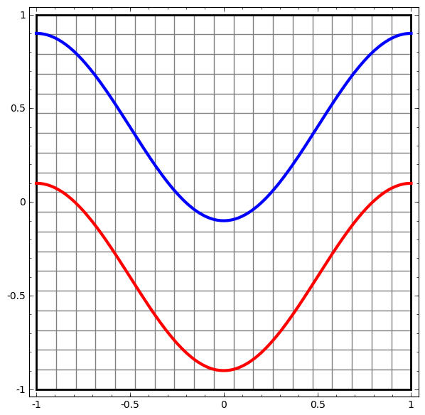
An obvious way to visualize the behavior of a neural network is to see how the algorithm classifies all possible objects (in our example, points) from a data set.
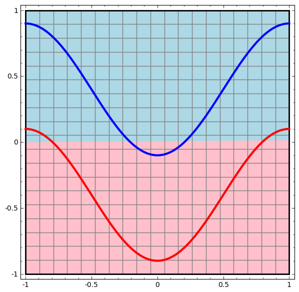
Let's start with the simplest class of neural network, with one input and output layer. Such a network tries to separate the two classes of data, dividing them with a line.
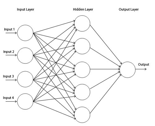
Such a network is not used in practice. Modern neural networks usually have several layers between their input and output, called "hidden" layers.
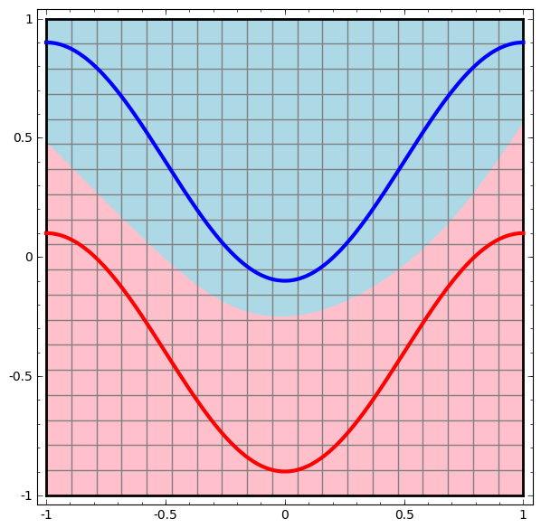
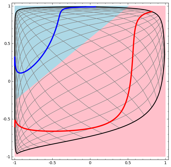
We visualize the behavior of this network, observing what it does with different points in its area. A network with a hidden layer separates the data with a more complex curve than a line.
With each layer, the network transforms the data, creating a new view. We can look at the data in each of these views and how the network with the hidden layer classifies them. When the algorithm reaches the final representation, the neural network will draw a line through the data (or, in higher dimensions, the hyperplane).
In the previous visualization, the data in the raw view is considered. You can imagine this by looking at the input layer. Now, consider it after it is transformed by the first layer. You can imagine this by looking at the hidden layer.
Each measurement corresponds to the activation of the neuron in the layer.
The hidden layer is trained on the presentation, so that the data are linearly separable.
Continuous visualization of layers
In the approach described in the previous section, we learn to understand networks by viewing the presentation corresponding to each layer. This gives us a discrete list of views.
The nontrivial part is to understand how we move from one to another. Fortunately, neural network levels have properties that make this possible.
There are many different types of layers used in neural networks.
Consider the tanh layer for a specific example. The tanh tanh (Wx + b) layer consists of:
We can imagine this as a continuous transformation as follows:
This principle of operation is very similar to other standard layers consisting of an affine transformation, followed by a point-by-point application of the monotone activation function.
This method can be used to understand more complex networks. So, the next network classifies two spirals, which are slightly entangled using four hidden layers. Over time, it is clear that the neural network is moving from a “raw” view to a higher level that the network has studied in order to classify the data. While the spirals are initially entangled, by the end they are linearly separable.
On the other hand, the following network, also using several levels, but cannot classify two spirals, which are more entangled.
It should be noted that these tasks are of limited complexity, because low-dimensional neural networks are used. If wider networks were used, problem solving would be easier.
Each layer stretches and compresses space, but it never cuts, breaks or folds it. Intuitively, we see that topological properties are preserved on each layer.
Such transformations that do not affect the topology are called homomorphisms (Wiki - This is a map of the algebraic system A, preserving the basic operations and the basic relations). Formally, they are bijections, which are continuous functions in both directions. In a bijective mapping, each element of one set corresponds to exactly one element of another set, and the inverse mapping is defined, which has the same property.
Theorem
Layers with N inputs and N conclusions are homomorphisms if the weight matrix W is not degenerate. (You need to be careful about the domain and range.)
Consider a two-dimensional data set with two classes A, B⊂R2:
A = {x | d (x, 0) <1/3}
B = {x | 2/3 <d (x, 0) <1}

A red, B blue
Requirement: a neural network cannot classify this dataset without having 3 or more hidden layers, regardless of width.
As mentioned earlier, a classification with a sigmoid function or a softmax layer is equivalent to trying to find a hyperplane (or in this case a line) that separates A and B in the final representation. Having only two hidden layers, the network is topologically unable to share data in this way, and is doomed to fail in this data set.
In the following visualization, we observe a hidden view while the network is training along with the classification line.
For this network, training is not enough to achieve one hundred percent result.
The algorithm falls into an unproductive local minimum, but is able to achieve ~ 80% of the classification accuracy.
In this example there was only one hidden layer, but it did not work.
Statement. Either each layer is a homomorphism, or the weight matrix of the layer has determinant 0.
If we add a third hidden item, the problem will become trivial. The neural network recognizes the following view: The
view makes it possible to share datasets with a hyperplane.
To better understand what is going on, let's consider an even simpler data set that is one-dimensional:
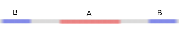
A = [- 1 / 3.1 / 3]
B = [- 1, −2 / 3] ∪ [2 / 3.1]
Without using a layer of two or more hidden elements, we cannot classify this dataset. But, if we use a network with two elements, we will learn to present the data as a good curve that allows us to separate classes using a line:
What's happening? One hidden item learns to fire when x> -1/2, and one learns to fire when x> 1/2. When the first one works, but not the second one, we know that we are in A.
Does this apply to real-world data sets, such as image sets? If you are serious about the hypothesis of diversity, I think it matters.
The multidimensional hypothesis is that the natural data form low-dimensional manifolds in the implantation space. There are both theoretical [1] and experimental [2] reasons for believing that this is true. If so, then the task of the classification algorithm is to separate the bundle of entangled manifolds.
In the previous examples, one class completely surrounded the other. Nevertheless, it is unlikely that the variety of images of dogs is completely surrounded by a collection of images of cats. But there are other more plausible topological situations that may still arise, as we will see in the next section.
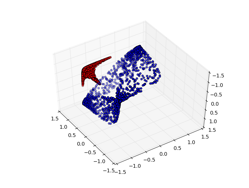
Another interesting data set is two connected tori A and B.
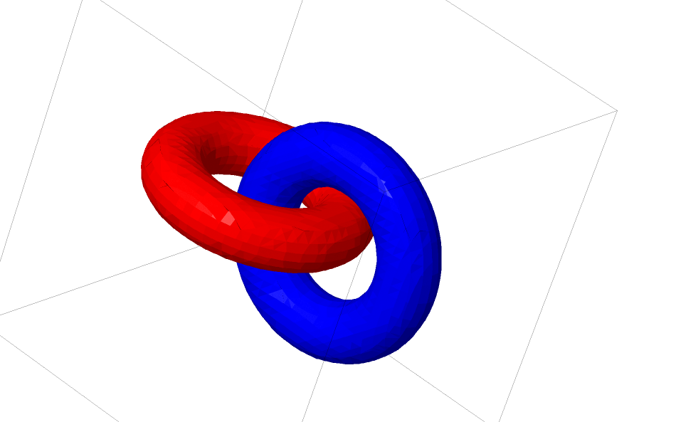
Like the previous data sets that we reviewed, this data set cannot be divided without using n + 1 dimensions, namely the fourth dimension.
Relationships are studied in knot theory, topology areas. Sometimes, when we see a connection, it is not immediately clear whether this is incoherence (a lot of things that are entangled together, but can be separated by continuous deformation) or not.
Relatively simple incoherence.
If a neural network using layers with only three units can classify it, then it is incoherent. (Question: Can all inconsistencies be classified on a network with only three inconsistencies, theoretically?)
From the point of view of this node, continuous visualization of the representations created by the neural network is a procedure for disentangling connections. In topology, we will call this ambient isotopy between the original link and the separated ones.
Formally, the isotopy of the surrounding space between the varieties A and B is a continuous function F: [0,1] × X → Y such that each Ft is a homeomorphism from X to its range, F0 is the identity function, and F1 maps A to B. T . Ft continuously goes from A to itself, to A to B.
Theorem: there is an isotopy of the surrounding space between the input and the network layer representation if: a) W is not degenerate, b) we are ready to transfer neurons to the hidden layer and c) there is more than 1 hidden item.
Until now, such connections, which we have talked about, are unlikely to appear in real data, but there are generalizations of a higher level. It is plausible that such features may exist in real data.
Links and nodes are one-dimensional manifolds, but we need 4 dimensions so that networks can unravel all of them. Similarly, even higher dimensional space may be required to be able to decompose n-dimensional manifolds. All n-dimensional manifolds can be expanded in 2n + 2 dimensions. [3]
The simple way is to try to pull the manifolds apart and stretch the pieces that are as confusing as possible. Although this will not be close to a genuine solution, such a solution can achieve relatively high classification accuracy and be an acceptable local minimum.

Such local minima are absolutely useless in terms of trying to solve topological problems, but topological problems can provide good motivation to study these problems.
On the other hand, if we are only interested in achieving good classification results, the approach is acceptable. If the tiny bit of the data manifold caught on to the other manifold, is this a problem? It is likely that arbitrarily good classification results will be obtained, despite this problem.
Improved layers for manipulating manifolds?
It is hard to imagine that standard affine transformed layers are really good for manipulating manifolds.
Perhaps it makes sense to have a completely different layer, which we can use in a composition with more traditional ones?
It is promising to study the vector field with the direction in which we want to shift the manifold:

And then we deform the space based on the vector field:
We could study the vector field at fixed points (just take some fixed points from the test data for use as anchors) and somehow interpolate.
Where v0 and v1 are vectors, and f0 (x) and f1 (x) are n-dimensional Gaussians.
Linear separability can be a huge and possibly unreasonable need for neural networks. It is natural to use the method of k-nearest neighbors (k-NN). However, the success of k-NN is largely dependent on the presentation that it classifies, so a good presentation is required before k-NN can work well.
k-nn is differentiable with respect to the representation on which it acts. Thus, we can directly train the network for k-NN classification. This can be viewed as a sort of “closest neighbor” layer, which acts as an alternative to softmax.
We do not want to pre-manage our entire set of workouts for each mini-party, because this will be a very expensive procedure. An adapted approach is to classify each element of the mini-batch based on the classes of other elements of the mini-batch, giving each unit weight divided by the distance from the classification goal.
Unfortunately, even with a complex architecture, using k-NN reduces the likelihood of error — and using simpler architectures worsens the results.
Topological properties of data, such as relationships, may make it impossible to linearly divide classes using low-dimensional networks, regardless of depth. Even in cases where it is technically possible. For example, spirals, which can be very difficult to separate.
For accurate data classification, neural networks need broad layers. In addition, the traditional layers of the neural network are poorly suited to represent important manipulations with manifolds; even if we set the weights manually, it would be difficult to compactly represent the transformations we want.
Understanding the behavior of deep neural networks in general is not a trivial task. It is easier to explore low-dimensional deep neural networks — networks in which there are only a few neurons in each layer. For low-dimensional networks, you can create visualizations to understand the behavior and training of such networks. This perspective will provide a deeper understanding of the behavior of neural networks and observe the connection that unites neural networks with the area of mathematics called topology.
From this follows a number of interesting things, including the fundamental lower bounds of the complexity of a neural network that is able to classify certain data sets.
Consider the principle of the network on the example
Let's start with a simple data set - two curves on a plane. The task of the network will learn to classify the belonging of points to curves.
An obvious way to visualize the behavior of a neural network is to see how the algorithm classifies all possible objects (in our example, points) from a data set.
Let's start with the simplest class of neural network, with one input and output layer. Such a network tries to separate the two classes of data, dividing them with a line.
Such a network is not used in practice. Modern neural networks usually have several layers between their input and output, called "hidden" layers.
Simple network diagram
We visualize the behavior of this network, observing what it does with different points in its area. A network with a hidden layer separates the data with a more complex curve than a line.
With each layer, the network transforms the data, creating a new view. We can look at the data in each of these views and how the network with the hidden layer classifies them. When the algorithm reaches the final representation, the neural network will draw a line through the data (or, in higher dimensions, the hyperplane).
In the previous visualization, the data in the raw view is considered. You can imagine this by looking at the input layer. Now, consider it after it is transformed by the first layer. You can imagine this by looking at the hidden layer.
Each measurement corresponds to the activation of the neuron in the layer.
The hidden layer is trained on the presentation, so that the data are linearly separable.
Continuous visualization of layers
In the approach described in the previous section, we learn to understand networks by viewing the presentation corresponding to each layer. This gives us a discrete list of views.
The nontrivial part is to understand how we move from one to another. Fortunately, neural network levels have properties that make this possible.
There are many different types of layers used in neural networks.
Consider the tanh layer for a specific example. The tanh tanh (Wx + b) layer consists of:
- Linear transformation by weight matrix W
- Translation using vector b
- Dotted tanh.
We can imagine this as a continuous transformation as follows:
This principle of operation is very similar to other standard layers consisting of an affine transformation, followed by a point-by-point application of the monotone activation function.
This method can be used to understand more complex networks. So, the next network classifies two spirals, which are slightly entangled using four hidden layers. Over time, it is clear that the neural network is moving from a “raw” view to a higher level that the network has studied in order to classify the data. While the spirals are initially entangled, by the end they are linearly separable.
On the other hand, the following network, also using several levels, but cannot classify two spirals, which are more entangled.
It should be noted that these tasks are of limited complexity, because low-dimensional neural networks are used. If wider networks were used, problem solving would be easier.
Tang layer topology
Each layer stretches and compresses space, but it never cuts, breaks or folds it. Intuitively, we see that topological properties are preserved on each layer.
Such transformations that do not affect the topology are called homomorphisms (Wiki - This is a map of the algebraic system A, preserving the basic operations and the basic relations). Formally, they are bijections, which are continuous functions in both directions. In a bijective mapping, each element of one set corresponds to exactly one element of another set, and the inverse mapping is defined, which has the same property.
Theorem
Layers with N inputs and N conclusions are homomorphisms if the weight matrix W is not degenerate. (You need to be careful about the domain and range.)
Evidence:
1. Предположим, что W имеет ненулевой детерминант. Тогда это биективная линейная функция с линейным обратным. Линейные функции непрерывны. Итак, умножение на W является гомеоморфизмом.
2. Отображения — гомоморфизмы
3. tanh (и сигмоиды и softplus, но не ReLU) являются непрерывными функциями с непрерывными обратными. Они являются биекциями, если мы внимательно относимся к области и диапазону, который мы рассматриваем. Применение их поточечно, является гомоморфизмом.
Таким образом, если W имеет ненулевой детерминант, слой является гомеоморфным.
Topology and classification
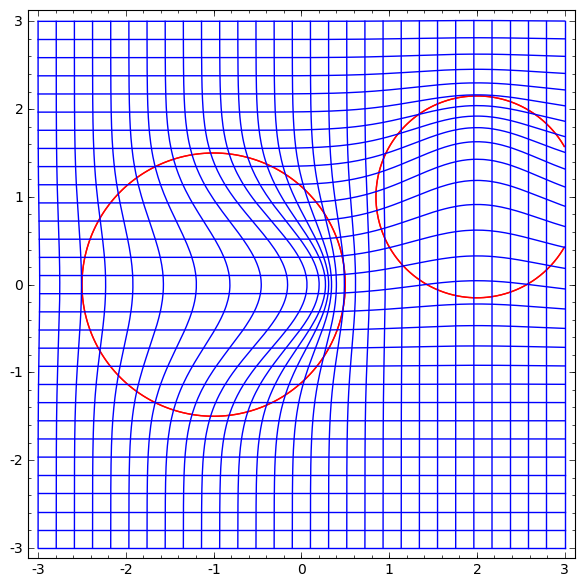
Consider a two-dimensional data set with two classes A, B⊂R2:
A = {x | d (x, 0) <1/3}
B = {x | 2/3 <d (x, 0) <1}
A red, B blue
Requirement: a neural network cannot classify this dataset without having 3 or more hidden layers, regardless of width.
As mentioned earlier, a classification with a sigmoid function or a softmax layer is equivalent to trying to find a hyperplane (or in this case a line) that separates A and B in the final representation. Having only two hidden layers, the network is topologically unable to share data in this way, and is doomed to fail in this data set.
In the following visualization, we observe a hidden view while the network is training along with the classification line.
For this network, training is not enough to achieve one hundred percent result.
The algorithm falls into an unproductive local minimum, but is able to achieve ~ 80% of the classification accuracy.
In this example there was only one hidden layer, but it did not work.
Statement. Either each layer is a homomorphism, or the weight matrix of the layer has determinant 0.
Evidence:
Если это гомоморфизм, то A по-прежнему окружен B, и линия не может их разделить. Но предположим, что она имеет детерминант 0: тогда набор данных коллапсирует на некоторой оси. Поскольку мы имеем дело с чем-то, гомеоморфным исходному набору данных, A окруженных B, и коллапсирование на любой оси означает, что мы будем иметь некоторые точки из A и B смешенными, и что приводит к невозможности для различения.
If we add a third hidden item, the problem will become trivial. The neural network recognizes the following view: The
view makes it possible to share datasets with a hyperplane.
To better understand what is going on, let's consider an even simpler data set that is one-dimensional:
A = [- 1 / 3.1 / 3]
B = [- 1, −2 / 3] ∪ [2 / 3.1]
Without using a layer of two or more hidden elements, we cannot classify this dataset. But, if we use a network with two elements, we will learn to present the data as a good curve that allows us to separate classes using a line:
What's happening? One hidden item learns to fire when x> -1/2, and one learns to fire when x> 1/2. When the first one works, but not the second one, we know that we are in A.
Diversity hypothesis
Does this apply to real-world data sets, such as image sets? If you are serious about the hypothesis of diversity, I think it matters.
The multidimensional hypothesis is that the natural data form low-dimensional manifolds in the implantation space. There are both theoretical [1] and experimental [2] reasons for believing that this is true. If so, then the task of the classification algorithm is to separate the bundle of entangled manifolds.
In the previous examples, one class completely surrounded the other. Nevertheless, it is unlikely that the variety of images of dogs is completely surrounded by a collection of images of cats. But there are other more plausible topological situations that may still arise, as we will see in the next section.
Connections and homotopies
Another interesting data set is two connected tori A and B.
Like the previous data sets that we reviewed, this data set cannot be divided without using n + 1 dimensions, namely the fourth dimension.
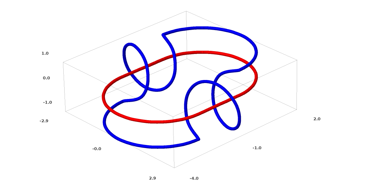
Relationships are studied in knot theory, topology areas. Sometimes, when we see a connection, it is not immediately clear whether this is incoherence (a lot of things that are entangled together, but can be separated by continuous deformation) or not.
Relatively simple incoherence.
If a neural network using layers with only three units can classify it, then it is incoherent. (Question: Can all inconsistencies be classified on a network with only three inconsistencies, theoretically?)
From the point of view of this node, continuous visualization of the representations created by the neural network is a procedure for disentangling connections. In topology, we will call this ambient isotopy between the original link and the separated ones.
Formally, the isotopy of the surrounding space between the varieties A and B is a continuous function F: [0,1] × X → Y such that each Ft is a homeomorphism from X to its range, F0 is the identity function, and F1 maps A to B. T . Ft continuously goes from A to itself, to A to B.
Theorem: there is an isotopy of the surrounding space between the input and the network layer representation if: a) W is not degenerate, b) we are ready to transfer neurons to the hidden layer and c) there is more than 1 hidden item.
Evidence:
1. Самая сложная часть — линейное преобразование. Чтобы это было возможно, нам нужно, чтобы W обладала положительным определителем. Наша предпосылка заключается в том, что она не равна нулю, и мы можем перевернуть знак, если он отрицательный, переключив два скрытых нейрона, и поэтому можем гарантировать, что определитель положителен. Пространство положительных детерминантных матриц является связным, поэтому существует p: [0,1] → GLn ®5 такое, что p (0) = Id и p (1) = W. Мы можем непрерывно переходить от функции тождества к W-преобразованию с помощью функции x → p (t) x, умножая x в каждой точке времени t на непрерывно переходящую матрицу p (t).
2. Мы можем непрерывно переходить от функции тождества к b-отображению с помощью функции x → x + tb.
3. Мы можем непрерывно переходить от тождественной функции к поточечному использованию σ с функцией: x → (1-t) x + tσ (x)
2. Мы можем непрерывно переходить от функции тождества к b-отображению с помощью функции x → x + tb.
3. Мы можем непрерывно переходить от тождественной функции к поточечному использованию σ с функцией: x → (1-t) x + tσ (x)
Until now, such connections, which we have talked about, are unlikely to appear in real data, but there are generalizations of a higher level. It is plausible that such features may exist in real data.
Links and nodes are one-dimensional manifolds, but we need 4 dimensions so that networks can unravel all of them. Similarly, even higher dimensional space may be required to be able to decompose n-dimensional manifolds. All n-dimensional manifolds can be expanded in 2n + 2 dimensions. [3]
Easy exit
The simple way is to try to pull the manifolds apart and stretch the pieces that are as confusing as possible. Although this will not be close to a genuine solution, such a solution can achieve relatively high classification accuracy and be an acceptable local minimum.
Such local minima are absolutely useless in terms of trying to solve topological problems, but topological problems can provide good motivation to study these problems.
On the other hand, if we are only interested in achieving good classification results, the approach is acceptable. If the tiny bit of the data manifold caught on to the other manifold, is this a problem? It is likely that arbitrarily good classification results will be obtained, despite this problem.
Improved layers for manipulating manifolds?
It is hard to imagine that standard affine transformed layers are really good for manipulating manifolds.
Perhaps it makes sense to have a completely different layer, which we can use in a composition with more traditional ones?
It is promising to study the vector field with the direction in which we want to shift the manifold:
And then we deform the space based on the vector field:
We could study the vector field at fixed points (just take some fixed points from the test data for use as anchors) and somehow interpolate.
The vector field above has the form:
Р (х) =( v0f0 (х) + v1f1 (х) )/( 1 + 0 (х) + f1 (х))
Where v0 and v1 are vectors, and f0 (x) and f1 (x) are n-dimensional Gaussians.
K-Nearest Neighbor Layers
Linear separability can be a huge and possibly unreasonable need for neural networks. It is natural to use the method of k-nearest neighbors (k-NN). However, the success of k-NN is largely dependent on the presentation that it classifies, so a good presentation is required before k-NN can work well.
k-nn is differentiable with respect to the representation on which it acts. Thus, we can directly train the network for k-NN classification. This can be viewed as a sort of “closest neighbor” layer, which acts as an alternative to softmax.
We do not want to pre-manage our entire set of workouts for each mini-party, because this will be a very expensive procedure. An adapted approach is to classify each element of the mini-batch based on the classes of other elements of the mini-batch, giving each unit weight divided by the distance from the classification goal.
Unfortunately, even with a complex architecture, using k-NN reduces the likelihood of error — and using simpler architectures worsens the results.
Conclusion
Topological properties of data, such as relationships, may make it impossible to linearly divide classes using low-dimensional networks, regardless of depth. Even in cases where it is technically possible. For example, spirals, which can be very difficult to separate.
For accurate data classification, neural networks need broad layers. In addition, the traditional layers of the neural network are poorly suited to represent important manipulations with manifolds; even if we set the weights manually, it would be difficult to compactly represent the transformations we want.
References to sources and explanations
[1] A lot of the natural transformations you might want to perform on an image, like translating or scaling an object in it, or changing the lighting, would form continuous curves in image space if you performed them continuously.
[2] Carlsson et al. found that local patches of images form a klein bottle.
[3] This result is mentioned in Wikipedia’s subsection on Isotopy versions.
[2] Carlsson et al. found that local patches of images form a klein bottle.
[3] This result is mentioned in Wikipedia’s subsection on Isotopy versions.