Calculation of the intensity of the telephone load in the KSC QUANT-E
Good afternoon. I would like to share with you information on calculating the intensity of telephone load in the KVANT-E CSK. This information will be useful for both professionals in this field, beginner students and just anyone interested in digital switching systems.
The data for the calculation are taken at random and are used as an example.
And do not be alarmed by the formulas, in fact, such a calculation will take no more than 15 minutes.
So, let's begin.
Categories of load sources differ in the intensity of specific subscriber loads. The assignment adopted 3 categories:
-subscribers of the business sector - category 1;
- subscribers of the housing sector - category 2;
-universal payphones - category 3.
The structure of subscribers by category for existing RATS is determined depending on the proportion of subscribers of the apartment sector, because payphones are allocated in a separate group. Therefore:
Ni, k = KкNi, and
where Ni, and is the number of individual subscribers;
Kк– the share of subscribers of the apartment sector.
The number of subscribers in the business sector is equal to the difference:
Ni, d = (1 - Kk) Ni, and the
structure of the CSK is determined minus universal payphones.
The number of individual telephones is:
N0, and = N0 - N0, t.
Knowing the number of individual SLTs, it is possible to determine the number of subscribers of the business sector (Nd) and apartment sector (Nk) using the formulas.
For each PBX, we determine the number of residential and business sector subscribers:
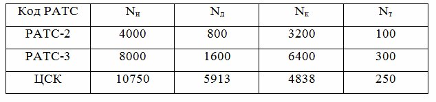
for RATS-2Nk = 0.80 • 4000 = 3200 numbers; Nd = 4000 - 3200 = 800 subscribers.
for RATS-3 Nk = 0.80 • 8000 = 6400 numbers; Nd = 8000 - 6400 = 1600 subscribers.
for CSKNk = (11000 - 250) • 0.45 = 4838 subscribers; Nd = 10750–4838 = 5913 subscribers.
The calculation results will be listed in Table 1.
Table 1 - The number of SLTs by category for all stations in the network.
The load intensities on the CSK are determined by the following formulas:
Y and АB j = Nyyd + Nkyyk + Nuit
Y in battery j = Ndyvd + Nkyvk Ymi
battery j = Ndymid + Nkymic + Ntummit Ymv
battery j = Ndymvd + Nkymvk
Calculation of subscriber loads for CSK:
Y and AB TsSK = 5913 • 0,074 + 4838 • 0,025 + 250 • 0,090 = 581,01
Y in AB CSK = 5913 • 0.070 + 4838 • 0.023 = 525.19 Earl
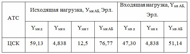
Ymi AB CSK = 5913 • 0.010 + 4838 • 0.001 + 250 • 0.050 = 76.77 Earl
Ymv AB CSK = 5913 • 0.008 + 4838 • 0.001 = 51.14 Earl
Perform subscriber load calculation for RATS-2:
Y and RATS-2 AB = 800 • 0.074 + 4838 • 0.025 + 100 • 0.090 = 189.15 Earl
YAT RATS-2 AB = 800 • 0.070 + 4838 • 0.023 = 167.27 Earl
Perform the calculation of subscriber loads for RATS-3:
Y and AB RATS-3 = 1600 • 0.074 + 6400 • 0.025 + 300 • 0.090 = 305.4 Earl
Y in AB RATS-3 = 1600 • 0.070 + 6400 • 0.023 = 259.2 Earl.
The calculation results are summarized in Table 2 and 3.
Table 2 - Calculation of the load.
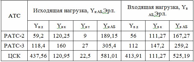
Table 3 - Calculation of the long-distance load
. subscriber load:
YиSPj = KspYiАБj
where Ksp. = 0.03 ÷ 0.05 - the proportion of the load that is sent to the special services.
Y and sp. CSK = 0.03 • 581.01 = 17.43 Earl
The intensity of the remaining outgoing load is determined by:
Yout ABJ = Y and ABA
Yispj Yout. AB CSK = 681.01 - 17.43 = 633.58 Earl
External outgoing loads from the AM to the group paths of the YGT AM are less than the load of the subscriber lines due to the difference in the time of occupation of the AL and the GT lines. Similarly, for analog exchanges, the load of the output of the GI of the incoming load. This difference is determined by the coefficient q, the value of which depends on the type of connection:
where ti is the average AL class occupation time for
Kk tco is the average duration of the station signal, tco = 3 s
tu is the connection setup time, ty = 0
tnab is the dialing time, which depends on the transmission method of the number from the TA:
- for the pulse method (DCS) tnab. = 1.5 n;
- for the frequency method (DTMF) tnab. = 0.4 n;
where n is the number of digits dialed and depends on the importance of numbering on the network.
For outgoing communication, the value n = 5 or 6, depending on the significance of the numbering. With mixed numbering
, the weighted average value n is determined: n = p5 5 + (1 - p5) 6, where p5 is the proportion of calls routed to the RATS with 5-digit numbering.
The value of p5 is equal to:
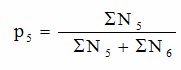
where ΣN5 and ΣN6 are the total capacity of the RATS, respectively, with 5 and 6-digit
numbers.
whence:
n = 0.52 • 5 + (1 - 0.52) • 6 = 5.48
tnab. = 1.5 • 5.48 = 8.22 s
tn = 3 + 8.22 + 0 = 11.22 s
For outgoing long-distance communication, the value of n is equal to:
n = pzone 9 + pmg 11 + pmn 14
where pzone. = 0.6 - the proportion of calls during zone communication;
pmg = 0.3 - the proportion of calls for long distance calls;
pm = 0.1 - the proportion of calls in international communications.
n = 0.6 • 9 + 0.3 • 11 + 0.1 • 14 = 10.1
tnab.m = 1.5 • 10.1 = 15.15 s
tnm = 3 + 15.15 + 0 = 18 , 15 s.
The coefficient qmi is equal to:
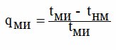
where tmi = 72po Kts – 0.5

For special services, qsp is equal to:

where tsp = 30 s is the reference time;
tn.sp = tco + 1.5n = 3 + 1.5 • 2 = 6 s - dialing time for the number of dialed digits equal to 2.

With incoming communication to the CSK, the reception of the number and the establishment of the connection are very small both with local and long-distance communication, therefore:
qin. = 1, qin. = qm in. = 1
For incoming communication on analog RATS, Y.in.i calculation is made taking into account the type of station:
- for a decade-step RATS when receiving a DCBI number (tND = 7 s), then:

- for a coordinate RATS when receiving a number with an MSC code (tNK = 2 c):
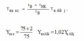
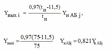
With outgoing communication on analog RATS Yout. i is equal to:
Calculation of external loads on existing RATS
Outgoing load:
- RATS-2, LH: Yout.2 = 0.821 • 189.15 = 155.29 Earl
- RATS-3, CS: Yout.3 = 0.821 • 305.4 = 250.73 Earl
Incoming load:
- RATS-2, LH: Yin.2 = 1.09 • 167.27 = 182.32 Earl
- RATS-3, CS: Yin.3 = 1.02 • 259.2 = 264 38 Earl
External loads on the group path, taking into account the difference in occupation of AL and GT, are respectively equal to:
- load on special services:
Ysp CSK = qspYisp CSK
where qsp = 0.8
Ysp. CSK = 0.8 • 17.43 = 13.94 Earl
- the output load of the switching field of the CSK is determined by the formula:
Yout CSK = q and Yvy AB CSK
Yvy TsSK = 0.83 • 581.01 = 482.24 Earl
- incoming load:
Yin TsSK = Yin AB
TsSK Yvkh TsSK = 525.19 Erl
- for long-distance communication:
YZSLTSSK = qmiYmi ABTSSK
YZSLTSSK = 0.74 • 76.77 = 56.81 Earl
YSLMTSSK = YmvABTSSK YSLM
TsSK = 51.14 Earl
YGTAM = YSPTSSK + Y and TsSKK + Yin. CSK + YZSLTSSK + YSLMTSSK
YGTAM = 13.94 + 482.24 + 525.19 + 56.81 + 51.14 = 1129.32 Earl The
inter-station load from station j to station k is determined by the formula:
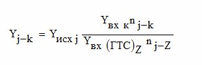
where Y ex. j is the intensity of the load coming from RATSj (CSK),
Yin.k is the intensity of the incoming load to RATSk,
Yin. (GTS) z - the sum of the loads included in all RATS, CSK, normalized by gravity coefficients relative to RATSj,
nj-k is the normalized coefficient of gravity from station j to station k.
After calculating the external loads on the CSK, RATSj, RATSk, the calculation data are entered into table 4 of the intensity of the outgoing and incoming network loads (Earl).
Table 4 - Intensities of the outgoing and incoming network loads (Earl):
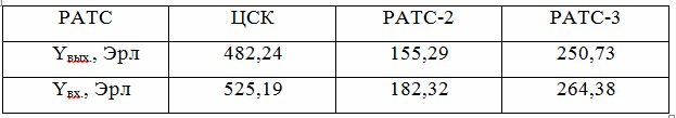
Table 5 - Gravity coefficients between the RATS:
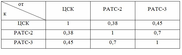
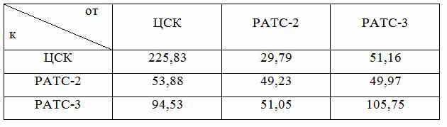
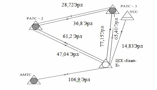
Using the above formula, we calculate the distribution of the outgoing load from the CSC to the network stations (Y0 - 0, Y0 - 2, Y0 - 3). The in-plant load Y0 - 0 is equal to:
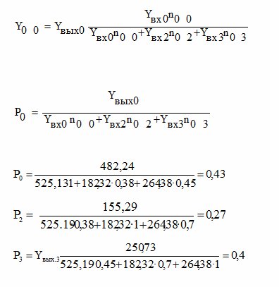
Then the in-
station load: Y0 - 0 = 0.43 • 525.19 • 1 = 225.83 Earl
Y0 - 2 = 0.43 • 182.32 • 0.38 = 29.79 Earl
Y0 - 3 = 0.43 • 264.38 • 0.45 = 51.16 Earl
Y2-0 = 0.27 • 525.19 • 0.38 = 53.88
Earl Y2-2 = 0.27 • 182.32 • 1 = 49 23 Earl
Y2-3 = 0.27 • 264.38 • 0.7 = 49.97 Earl
Y3-0 = 0.4 • 525.19 • 0.45 = 94.53
Earl Y3-2 = 0.4 • 182.32 • 0.7 = 51.05 Earl
Y3-3 = 0.4 • 264.38 • 1 = 105.75 Earl
Table 6 - Intensity of the inter-station load, Earl
The results of calculation of loads on CSK are entered on the load distribution diagram for AM and UKS CSK:
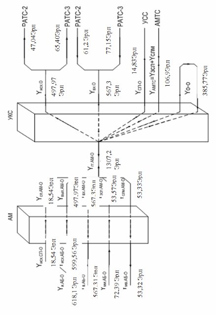
Load on SL beams is determined by the results of calculating the inter-station loads (table 10), taking into account the load coming from the digital system to the CSS and automatic telephone exchange. To determine the load on the SL beams, a load
distribution diagram is depicted. Load distribution on the GTS:
That's all. In fact, everything is simpler than it seems at first glance.
I hope that my efforts will benefit someone.
The data for the calculation are taken at random and are used as an example.
And do not be alarmed by the formulas, in fact, such a calculation will take no more than 15 minutes.
So, let's begin.
Calculation of the intensity of the telephone load
Categories of load sources differ in the intensity of specific subscriber loads. The assignment adopted 3 categories:
-subscribers of the business sector - category 1;
- subscribers of the housing sector - category 2;
-universal payphones - category 3.
The structure of subscribers by category for existing RATS is determined depending on the proportion of subscribers of the apartment sector, because payphones are allocated in a separate group. Therefore:
Ni, k = KкNi, and
where Ni, and is the number of individual subscribers;
Kк– the share of subscribers of the apartment sector.
The number of subscribers in the business sector is equal to the difference:
Ni, d = (1 - Kk) Ni, and the
structure of the CSK is determined minus universal payphones.
The number of individual telephones is:
N0, and = N0 - N0, t.
Knowing the number of individual SLTs, it is possible to determine the number of subscribers of the business sector (Nd) and apartment sector (Nk) using the formulas.
For each PBX, we determine the number of residential and business sector subscribers:
for RATS-2Nk = 0.80 • 4000 = 3200 numbers; Nd = 4000 - 3200 = 800 subscribers.
for RATS-3 Nk = 0.80 • 8000 = 6400 numbers; Nd = 8000 - 6400 = 1600 subscribers.
for CSKNk = (11000 - 250) • 0.45 = 4838 subscribers; Nd = 10750–4838 = 5913 subscribers.
The calculation results will be listed in Table 1.
Table 1 - The number of SLTs by category for all stations in the network.
The load intensities on the CSK are determined by the following formulas:
Y and АB j = Nyyd + Nkyyk + Nuit
Y in battery j = Ndyvd + Nkyvk Ymi
battery j = Ndymid + Nkymic + Ntummit Ymv
battery j = Ndymvd + Nkymvk
Calculation of subscriber loads for CSK:
Y and AB TsSK = 5913 • 0,074 + 4838 • 0,025 + 250 • 0,090 = 581,01
Y in AB CSK = 5913 • 0.070 + 4838 • 0.023 = 525.19 Earl
Ymi AB CSK = 5913 • 0.010 + 4838 • 0.001 + 250 • 0.050 = 76.77 Earl
Ymv AB CSK = 5913 • 0.008 + 4838 • 0.001 = 51.14 Earl
Perform subscriber load calculation for RATS-2:
Y and RATS-2 AB = 800 • 0.074 + 4838 • 0.025 + 100 • 0.090 = 189.15 Earl
YAT RATS-2 AB = 800 • 0.070 + 4838 • 0.023 = 167.27 Earl
Perform the calculation of subscriber loads for RATS-3:
Y and AB RATS-3 = 1600 • 0.074 + 6400 • 0.025 + 300 • 0.090 = 305.4 Earl
Y in AB RATS-3 = 1600 • 0.070 + 6400 • 0.023 = 259.2 Earl.
The calculation results are summarized in Table 2 and 3.
Table 2 - Calculation of the load.
Table 3 - Calculation of the long-distance load
. subscriber load:
YиSPj = KspYiАБj
where Ksp. = 0.03 ÷ 0.05 - the proportion of the load that is sent to the special services.
Y and sp. CSK = 0.03 • 581.01 = 17.43 Earl
The intensity of the remaining outgoing load is determined by:
Yout ABJ = Y and ABA
Yispj Yout. AB CSK = 681.01 - 17.43 = 633.58 Earl
External outgoing loads from the AM to the group paths of the YGT AM are less than the load of the subscriber lines due to the difference in the time of occupation of the AL and the GT lines. Similarly, for analog exchanges, the load of the output of the GI of the incoming load. This difference is determined by the coefficient q, the value of which depends on the type of connection:
where ti is the average AL class occupation time for
Kk tco is the average duration of the station signal, tco = 3 s
tu is the connection setup time, ty = 0
tnab is the dialing time, which depends on the transmission method of the number from the TA:
- for the pulse method (DCS) tnab. = 1.5 n;
- for the frequency method (DTMF) tnab. = 0.4 n;
where n is the number of digits dialed and depends on the importance of numbering on the network.
For outgoing communication, the value n = 5 or 6, depending on the significance of the numbering. With mixed numbering
, the weighted average value n is determined: n = p5 5 + (1 - p5) 6, where p5 is the proportion of calls routed to the RATS with 5-digit numbering.
The value of p5 is equal to:
where ΣN5 and ΣN6 are the total capacity of the RATS, respectively, with 5 and 6-digit
numbers.
whence:
n = 0.52 • 5 + (1 - 0.52) • 6 = 5.48
tnab. = 1.5 • 5.48 = 8.22 s
tn = 3 + 8.22 + 0 = 11.22 s
For outgoing long-distance communication, the value of n is equal to:
n = pzone 9 + pmg 11 + pmn 14
where pzone. = 0.6 - the proportion of calls during zone communication;
pmg = 0.3 - the proportion of calls for long distance calls;
pm = 0.1 - the proportion of calls in international communications.
n = 0.6 • 9 + 0.3 • 11 + 0.1 • 14 = 10.1
tnab.m = 1.5 • 10.1 = 15.15 s
tnm = 3 + 15.15 + 0 = 18 , 15 s.
The coefficient qmi is equal to:
where tmi = 72po Kts – 0.5
For special services, qsp is equal to:
where tsp = 30 s is the reference time;
tn.sp = tco + 1.5n = 3 + 1.5 • 2 = 6 s - dialing time for the number of dialed digits equal to 2.
With incoming communication to the CSK, the reception of the number and the establishment of the connection are very small both with local and long-distance communication, therefore:
qin. = 1, qin. = qm in. = 1
For incoming communication on analog RATS, Y.in.i calculation is made taking into account the type of station:
- for a decade-step RATS when receiving a DCBI number (tND = 7 s), then:
- for a coordinate RATS when receiving a number with an MSC code (tNK = 2 c):
With outgoing communication on analog RATS Yout. i is equal to:
Calculation of external loads on existing RATS
Outgoing load:
- RATS-2, LH: Yout.2 = 0.821 • 189.15 = 155.29 Earl
- RATS-3, CS: Yout.3 = 0.821 • 305.4 = 250.73 Earl
Incoming load:
- RATS-2, LH: Yin.2 = 1.09 • 167.27 = 182.32 Earl
- RATS-3, CS: Yin.3 = 1.02 • 259.2 = 264 38 Earl
External loads on the group path, taking into account the difference in occupation of AL and GT, are respectively equal to:
- load on special services:
Ysp CSK = qspYisp CSK
where qsp = 0.8
Ysp. CSK = 0.8 • 17.43 = 13.94 Earl
- the output load of the switching field of the CSK is determined by the formula:
Yout CSK = q and Yvy AB CSK
Yvy TsSK = 0.83 • 581.01 = 482.24 Earl
- incoming load:
Yin TsSK = Yin AB
TsSK Yvkh TsSK = 525.19 Erl
- for long-distance communication:
YZSLTSSK = qmiYmi ABTSSK
YZSLTSSK = 0.74 • 76.77 = 56.81 Earl
YSLMTSSK = YmvABTSSK YSLM
TsSK = 51.14 Earl
YGTAM = YSPTSSK + Y and TsSKK + Yin. CSK + YZSLTSSK + YSLMTSSK
YGTAM = 13.94 + 482.24 + 525.19 + 56.81 + 51.14 = 1129.32 Earl The
inter-station load from station j to station k is determined by the formula:
where Y ex. j is the intensity of the load coming from RATSj (CSK),
Yin.k is the intensity of the incoming load to RATSk,
Yin. (GTS) z - the sum of the loads included in all RATS, CSK, normalized by gravity coefficients relative to RATSj,
nj-k is the normalized coefficient of gravity from station j to station k.
After calculating the external loads on the CSK, RATSj, RATSk, the calculation data are entered into table 4 of the intensity of the outgoing and incoming network loads (Earl).
Table 4 - Intensities of the outgoing and incoming network loads (Earl):
Table 5 - Gravity coefficients between the RATS:
Using the above formula, we calculate the distribution of the outgoing load from the CSC to the network stations (Y0 - 0, Y0 - 2, Y0 - 3). The in-plant load Y0 - 0 is equal to:
Then the in-
station load: Y0 - 0 = 0.43 • 525.19 • 1 = 225.83 Earl
Y0 - 2 = 0.43 • 182.32 • 0.38 = 29.79 Earl
Y0 - 3 = 0.43 • 264.38 • 0.45 = 51.16 Earl
Y2-0 = 0.27 • 525.19 • 0.38 = 53.88
Earl Y2-2 = 0.27 • 182.32 • 1 = 49 23 Earl
Y2-3 = 0.27 • 264.38 • 0.7 = 49.97 Earl
Y3-0 = 0.4 • 525.19 • 0.45 = 94.53
Earl Y3-2 = 0.4 • 182.32 • 0.7 = 51.05 Earl
Y3-3 = 0.4 • 264.38 • 1 = 105.75 Earl
Table 6 - Intensity of the inter-station load, Earl
The results of calculation of loads on CSK are entered on the load distribution diagram for AM and UKS CSK:
Load on SL beams is determined by the results of calculating the inter-station loads (table 10), taking into account the load coming from the digital system to the CSS and automatic telephone exchange. To determine the load on the SL beams, a load
distribution diagram is depicted. Load distribution on the GTS:
That's all. In fact, everything is simpler than it seems at first glance.
I hope that my efforts will benefit someone.