Basics of stereo vision
This article contains basic information about the mathematical apparatus used in stereo vision. The idea of writing it came about after I started working with stereo vision methods, in particular, using algorithms implemented in OpenCV . These algorithms often refer to various concepts, such as “fundamental matrix”, “epipolar geometry”, “triangulation”. There are very good books on computer vision, which describe, including stereo vision and all the necessary concepts, but they often contain too much information for a beginner. Here, in a short form, the basic information on how stereo vision works and the basic necessary concepts associated with it:
To understand the contents of the article, it is enough to have a general idea of analytic geometry and linear algebra: to know what a matrix, vector, scalar and vector product are.
For further discussion, we will mainly need an understanding of the analytical approach to projective geometry, and it is he who is presented below.
Points of the projective plane. Consider a two-dimensional projective space (also called a projective plane). While on the ordinary Euclidean plane, points are described by a pair of coordinates ( x , y) T , on the projective plane described by three-point vector ( x , y , w ) T . Moreover, for any nonzero number a , the vectors ( x , y , w ) T and ( ax , ay , aw ) T correspond to the same point. And the zero vector (0,0,0) T does not correspond to any point and is thrown out of consideration. Such a description of plane points is called homogeneous coordinates.
The points of the projective plane can be associated with the points of the ordinary Euclidean plane. Vector coordinate ( x , y , w ) T when w ≠ 0 associate point Euclidean plane with coordinates ( x / w , y / w ) T . If w = 0, i.e. the coordinate vector has the form ( x , y , 0 T ), then we say that this point is at infinity. Thus, the projective plane can be considered as a Euclidean plane supplemented by points from infinity.
Go from homogeneous coordinates (x , y , w ) T to conventional Euclidean possible by dividing coordinate vector of the latest component and its subsequent discarding ( x , y , w ) T → ( x / w , y / w ) T . And from Euclidean coordinates ( x , y ) T we can go over to homogeneous ones by supplementing the coordinate vector with one: ( x , y ) T → ( x , y , 1) T
Lines on the projective plane. Any line in the projective plane is described, like the point ternary vector l = ( a , b , c ) T . Again, the vector describing the line is determined up to a nonzero factor. Moreover, the equation of the line will have the form: l T x = 0.
In the case when a 2 + b 2 ≠ 0, we have an analog of the usual line ax + by + c = 0. And the vector (0,0, w ) corresponds to the straight line in infinity.
Three-dimensional projective space. By analogy with the projective plane, the projective points of the three-dimensional space defined by four-component vector of homogeneous coordinates ( x , y , z , w ) T . Again, for any nonzero number a , the coordinate vectors ( x , y , z , w ) T and ( ax , ay , az , aw ) T correspond to the same point.
As in the case of the projective plane, between the points of the three-dimensional Euclidean space and the three-dimensional projective space we can establish a correspondence. Vector of homogeneous coordinates ( x , y , z , w ) T when w ≠ 0 corresponds to the point Evklodova space with coordinates ( x / w , y / w , z / w ) T . And about a point with a vector of homogeneous coordinates of the form ( x , y , z , 0) T they say that it lies at infinity.
Projective transformation. Another thing that will be required for further presentation is projective transformations (homography, projective transformation - in the English literature). From a geometric point of view, a projective transformation is a reversible transformation of a projective plane (or space) that takes straight lines to straight lines. In coordinates, the projective transformation is expressed as a non-degenerate square matrix H , while the coordinate vector x goes into the coordinate vector x 'according to the following formula: x ' = H x .
The projection formula has a simple mathematical notation in homogeneous coordinates:
The matrix P is expressed as follows P = KR [ I | - c ] = K [ R | t ], where K is the upper triangular matrix of internal parameters of a 3 × 3 camera (a specific view is given below), R is an 3 × 3 orthogonal matrix that determines the rotation of the camera relative to the global coordinate system, I is a 3 × 3 identity matrix, vectorc - coordinates of the center of the camera, and t = - R c .
It should be noted that the camera matrix defined up to a nonzero constant multiplier, but the change points of the projection results by the formula x = P X . However, this constant factor is usually chosen so that the camera matrix has the form described above.
In the simplest case, when the center of the camera lies at the origin, the main axis of the camera is aligned with the Cz axis, the coordinate axes on the camera plane have the same scale (which is equivalent to square pixels), and the center of the image has zero coordinates, the camera matrix will be P = K [I | 0 ], where
In addition, due to the imperfection of optics, images received from cameras contain distortion distortions. These distortions have a nonlinear mathematical record:
Distortions do not depend on the distance to the object, but depend only on the coordinates of the points at which the pixels of the object are projected. Accordingly, in order to compensate for distortions, the original image obtained from the camera is usually converted. This transformation will be the same for all images received from the camera, provided that the focal length is constant (mathematically, the same matrix of internal parameters).
In a situation where the internal parameters of the camera are known and the distortion coefficients say that the camera is calibrated.
Matrices of a pair of cameras, calibration. Suppose there are two cameras defined by their matrices P and P 'in some coordinate system. In this case, they say that there are a couple of calibrated cameras. If the centers of the cameras do not match, then this pair of cameras can be used to determine the three-dimensional coordinates of the observed points.
Often, the coordinate system is chosen so that the camera matrices have the form P = K [ I | 0], P '= K ' [ R '| t']. This can always be done if you select the origin that coincides with the center of the first camera and direct the Z axis along its optical axis.
Calibration of cameras is usually performed by repeatedly shooting a calibration template; key points can easily be identified in the image for which their relative positions in space are known. Next, systems of equations are compiled and solved (approximately), linking the coordinates of the projections, the camera matrix and the position of the points of the template in space.
There are commonly available implementations of calibration algorithms, such as the Matlab Calibration toolbox . The OpenCV library also includes algorithms for calibrating cameras and searching for a calibration template in the image.
Epipolar geometry. Before proceeding to the description of the actual method of calculating the three-dimensional coordinates of points, I will describe some important geometric properties that relate the position of the projections of a point of three-dimensional space on images from both cameras.
Thus, to every point xin the image of the left camera corresponds to the epipolar line l 'in the image of the right camera. In this case, the pair for x in the image of the right camera can lie only on the corresponding epipolar line. Similarly, each point x 'in the right image corresponds to an epipolar line l on the left.
Epipolar geometry is used to search for stereopairs, and to verify that a pair of points can be a stereopair (i.e., a projection of some point in space).
Epipolar geometry has a very simple notation in coordinates. Let there be a pair of calibrated cameras, and let x be the uniform coordinates of a point in the image of one camera, and x'- in the image of the second. There exists a 3 × 3 matrix F such that a pair of points x , x 'is a stereo pair if and only if:
In the case when the camera arrays have the form P = K [ I | 0], P '= K ' [ R | t ] the fundamental matrix can be calculated by the formula:
In addition to the fundamental matrix, there is such a thing as an essential matrix: E = K ' T F K. In the case when the matrices of internal parameters are unity, the essential matrix will coincide with the fundamental. Using the essential matrix, you can restore the position and rotation of the second camera relative to the first, so it is used in tasks in which you need to determine the movement of the camera.
Triangulation of points (triangulation). Now let's move on to how to determine the three-dimensional coordinates of a point from the coordinates of its projections. This process is called triangulation in the literature.
Suppose there are two calibrated cameras with matrices P 1 and P 2 . x 1 and x 2 are the homogeneous projection coordinates of a point in the space X. Then you can make the following system of equations:
The idea behind building a depth map from a stereo pair is very simple. For each point in one image, it searches for a pair of points in another image. And by a pair of corresponding points, you can perform triangulation and determine the coordinates of their inverse image in three-dimensional space. Knowing the three-dimensional coordinates of the prototype, the depth is calculated as the distance to the plane of the camera.
The paired point must be sought on the epipolar line. Accordingly, to simplify the search, the images are aligned so that all the epipolar lines are parallel to the sides of the image (usually horizontal). Moreover, the images are aligned so that for a point with coordinates ( x 0 , y 0 ), the corresponding epipolar line is given by the equation x = x 0then for each point the corresponding pair point must be searched in the same line in the image from the second camera. This process of image alignment is called rectification. Typically, rectification is accomplished by remapping the image and combining it with getting rid of distortion. An example of rectified images is shown in Figure 3, the images are taken from the database of images comparing various methods for constructing a depth map http://vision.middlebury.edu/stereo .
- projective geometry and uniform coordinates
- camera model
- epipolar geometry (epiporal geomerty), fundamental and essential matrix (fundamental matrix, essential matrix)
- triangulation of a stereo pair of points
- depth map, disparity map, and the idea behind its calculation
To understand the contents of the article, it is enough to have a general idea of analytic geometry and linear algebra: to know what a matrix, vector, scalar and vector product are.
1 Projective geometry and homogeneous coordinates
Projective geometry plays a significant role in stereo vision geometry . There are several approaches to projective geometry: geometric (to introduce the concept of geometric objects like Euclidean geometry, axioms and from this to derive all the properties of a projective space), analytical (to consider everything in coordinates, as in an analytical approach to Euclidean geometry), algebraic.For further discussion, we will mainly need an understanding of the analytical approach to projective geometry, and it is he who is presented below.
Points of the projective plane. Consider a two-dimensional projective space (also called a projective plane). While on the ordinary Euclidean plane, points are described by a pair of coordinates ( x , y) T , on the projective plane described by three-point vector ( x , y , w ) T . Moreover, for any nonzero number a , the vectors ( x , y , w ) T and ( ax , ay , aw ) T correspond to the same point. And the zero vector (0,0,0) T does not correspond to any point and is thrown out of consideration. Such a description of plane points is called homogeneous coordinates.
The points of the projective plane can be associated with the points of the ordinary Euclidean plane. Vector coordinate ( x , y , w ) T when w ≠ 0 associate point Euclidean plane with coordinates ( x / w , y / w ) T . If w = 0, i.e. the coordinate vector has the form ( x , y , 0 T ), then we say that this point is at infinity. Thus, the projective plane can be considered as a Euclidean plane supplemented by points from infinity.
Go from homogeneous coordinates (x , y , w ) T to conventional Euclidean possible by dividing coordinate vector of the latest component and its subsequent discarding ( x , y , w ) T → ( x / w , y / w ) T . And from Euclidean coordinates ( x , y ) T we can go over to homogeneous ones by supplementing the coordinate vector with one: ( x , y ) T → ( x , y , 1) T
Lines on the projective plane. Any line in the projective plane is described, like the point ternary vector l = ( a , b , c ) T . Again, the vector describing the line is determined up to a nonzero factor. Moreover, the equation of the line will have the form: l T x = 0.
In the case when a 2 + b 2 ≠ 0, we have an analog of the usual line ax + by + c = 0. And the vector (0,0, w ) corresponds to the straight line in infinity.
Three-dimensional projective space. By analogy with the projective plane, the projective points of the three-dimensional space defined by four-component vector of homogeneous coordinates ( x , y , z , w ) T . Again, for any nonzero number a , the coordinate vectors ( x , y , z , w ) T and ( ax , ay , az , aw ) T correspond to the same point.
As in the case of the projective plane, between the points of the three-dimensional Euclidean space and the three-dimensional projective space we can establish a correspondence. Vector of homogeneous coordinates ( x , y , z , w ) T when w ≠ 0 corresponds to the point Evklodova space with coordinates ( x / w , y / w , z / w ) T . And about a point with a vector of homogeneous coordinates of the form ( x , y , z , 0) T they say that it lies at infinity.
Projective transformation. Another thing that will be required for further presentation is projective transformations (homography, projective transformation - in the English literature). From a geometric point of view, a projective transformation is a reversible transformation of a projective plane (or space) that takes straight lines to straight lines. In coordinates, the projective transformation is expressed as a non-degenerate square matrix H , while the coordinate vector x goes into the coordinate vector x 'according to the following formula: x ' = H x .
2 Projective camera model
Modern CCD cameras are well described using the following model, called a projective camera, pinhole camera. The projective camera is defined by the center of the camera , the main axis - the beam starting in the center of the camera and directed to where the camera is looking, the image plane - the plane onto which points are projected, and the coordinate system on this plane. In such a model, an arbitrary point in the space X is projected onto the image plane at the point x lying on the segment CX , which connects the center of the camera C with the starting point X (see Fig. 1).
Figure 1: Camera Model. C is the center of the camera, Cp is the main axis of the camera. Point X of three-dimensional space is projected to point x - on the image plane.
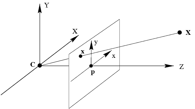
The projection formula has a simple mathematical notation in homogeneous coordinates:
where X is the homogeneous coordinates of a point in space, x is the homogeneous coordinates of a point in the plane, P is the matrix of a 3 × 4 camera.
x = P X
The matrix P is expressed as follows P = KR [ I | - c ] = K [ R | t ], where K is the upper triangular matrix of internal parameters of a 3 × 3 camera (a specific view is given below), R is an 3 × 3 orthogonal matrix that determines the rotation of the camera relative to the global coordinate system, I is a 3 × 3 identity matrix, vectorc - coordinates of the center of the camera, and t = - R c .
It should be noted that the camera matrix defined up to a nonzero constant multiplier, but the change points of the projection results by the formula x = P X . However, this constant factor is usually chosen so that the camera matrix has the form described above.
In the simplest case, when the center of the camera lies at the origin, the main axis of the camera is aligned with the Cz axis, the coordinate axes on the camera plane have the same scale (which is equivalent to square pixels), and the center of the image has zero coordinates, the camera matrix will be P = K [I | 0 ], where
In real CCD cameras, pixels usually differ slightly from square ones, and the center of the image has non-zero coordinates. In this case, the matrix of internal parameters will take the form:
The coefficients f , α x , α y - are called the focal lengths of the camera (respectively common and along the x and y axes ).
In addition, due to the imperfection of optics, images received from cameras contain distortion distortions. These distortions have a nonlinear mathematical record:
where k 1 , k 2 , p 1 , p 2 , k 3 are the distortion coefficients, which are the parameters of the optical system; r 2 = x ' 2 + y ' 2 ; ( x ', y ') - the coordinates of the projection of the point relative to the center of the image with square pixels and the absence of distortion; ( x ″, y ″) - distorted coordinates of a point relative to the center of the image in square pixels.

Distortions do not depend on the distance to the object, but depend only on the coordinates of the points at which the pixels of the object are projected. Accordingly, in order to compensate for distortions, the original image obtained from the camera is usually converted. This transformation will be the same for all images received from the camera, provided that the focal length is constant (mathematically, the same matrix of internal parameters).
In a situation where the internal parameters of the camera are known and the distortion coefficients say that the camera is calibrated.
3 pair of cameras
One can talk about determining the three-dimensional coordinates of observed points when there are at least two cameras.Matrices of a pair of cameras, calibration. Suppose there are two cameras defined by their matrices P and P 'in some coordinate system. In this case, they say that there are a couple of calibrated cameras. If the centers of the cameras do not match, then this pair of cameras can be used to determine the three-dimensional coordinates of the observed points.
Often, the coordinate system is chosen so that the camera matrices have the form P = K [ I | 0], P '= K ' [ R '| t']. This can always be done if you select the origin that coincides with the center of the first camera and direct the Z axis along its optical axis.
Calibration of cameras is usually performed by repeatedly shooting a calibration template; key points can easily be identified in the image for which their relative positions in space are known. Next, systems of equations are compiled and solved (approximately), linking the coordinates of the projections, the camera matrix and the position of the points of the template in space.
There are commonly available implementations of calibration algorithms, such as the Matlab Calibration toolbox . The OpenCV library also includes algorithms for calibrating cameras and searching for a calibration template in the image.
Epipolar geometry. Before proceeding to the description of the actual method of calculating the three-dimensional coordinates of points, I will describe some important geometric properties that relate the position of the projections of a point of three-dimensional space on images from both cameras.
Let there be two cameras, as shown in Figure 2. C is the center of the first camera, C 'is the center of the second camera. The point of space X is projected at x on the image plane of the left camera and at x 'on the image plane of the right camera. The prototype of the point x in the image of the left camera is the ray xX . This beam is projected onto the plane of the second chamber in a straight line l ', called the epipolar line. The image of point X on the image plane of the second camera necessarily lies on the epipolar line l '.
Figure 2: Epipolar Geometry

Thus, to every point xin the image of the left camera corresponds to the epipolar line l 'in the image of the right camera. In this case, the pair for x in the image of the right camera can lie only on the corresponding epipolar line. Similarly, each point x 'in the right image corresponds to an epipolar line l on the left.
Epipolar geometry is used to search for stereopairs, and to verify that a pair of points can be a stereopair (i.e., a projection of some point in space).
Epipolar geometry has a very simple notation in coordinates. Let there be a pair of calibrated cameras, and let x be the uniform coordinates of a point in the image of one camera, and x'- in the image of the second. There exists a 3 × 3 matrix F such that a pair of points x , x 'is a stereo pair if and only if:
The matrix F is called the fundamental matrix. Its rank is 2, it is determined up to a nonzero factor and depends only on the matrices of the source cameras P and P '.
x ' T F x = 0
In the case when the camera arrays have the form P = K [ I | 0], P '= K ' [ R | t ] the fundamental matrix can be calculated by the formula:
where for the vector e the notation [ e ] X is calculated as
Using the fundamental matrix, the equations of the epipolar lines are calculated. For the point x , the vector defining the epipolar line will have the form l '= F x , and the equation of the epipolar line itself will be l ' T x '= 0. Similarly for the point x ', the vector defining the epipolar line will have the form l = F T x '.
In addition to the fundamental matrix, there is such a thing as an essential matrix: E = K ' T F K. In the case when the matrices of internal parameters are unity, the essential matrix will coincide with the fundamental. Using the essential matrix, you can restore the position and rotation of the second camera relative to the first, so it is used in tasks in which you need to determine the movement of the camera.
Triangulation of points (triangulation). Now let's move on to how to determine the three-dimensional coordinates of a point from the coordinates of its projections. This process is called triangulation in the literature.
Suppose there are two calibrated cameras with matrices P 1 and P 2 . x 1 and x 2 are the homogeneous projection coordinates of a point in the space X. Then you can make the following system of equations:
In practice, the following approach is applied to solve this system. Vectorly multiply the first equation by x 1 , the second by x 2 , get rid of linearly dependent equations and bring the system to the form A X = 0, where A has a size of 4 × 4. Then we can either proceed from that that the vector X is the homogeneous coordinates of the point, put its last component equal to 1 and solve the resulting system of 3 equations with three unknowns. An alternative method - to take any non-zero solution of A X = 0, for example calculated as the singular vector corresponding to the smallest singular value of the matrix A .

4 Building a depth map
A depth map is an image on which, for each pixel, instead of color, its distance to the camera is stored. The depth map can be obtained using a special depth camera (for example, the Kinect sensor is a kind of such a camera), and it can also be constructed using a stereo pair of images.The idea behind building a depth map from a stereo pair is very simple. For each point in one image, it searches for a pair of points in another image. And by a pair of corresponding points, you can perform triangulation and determine the coordinates of their inverse image in three-dimensional space. Knowing the three-dimensional coordinates of the prototype, the depth is calculated as the distance to the plane of the camera.
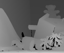
The paired point must be sought on the epipolar line. Accordingly, to simplify the search, the images are aligned so that all the epipolar lines are parallel to the sides of the image (usually horizontal). Moreover, the images are aligned so that for a point with coordinates ( x 0 , y 0 ), the corresponding epipolar line is given by the equation x = x 0then for each point the corresponding pair point must be searched in the same line in the image from the second camera. This process of image alignment is called rectification. Typically, rectification is accomplished by remapping the image and combining it with getting rid of distortion. An example of rectified images is shown in Figure 3, the images are taken from the database of images comparing various methods for constructing a depth map http://vision.middlebury.edu/stereo .
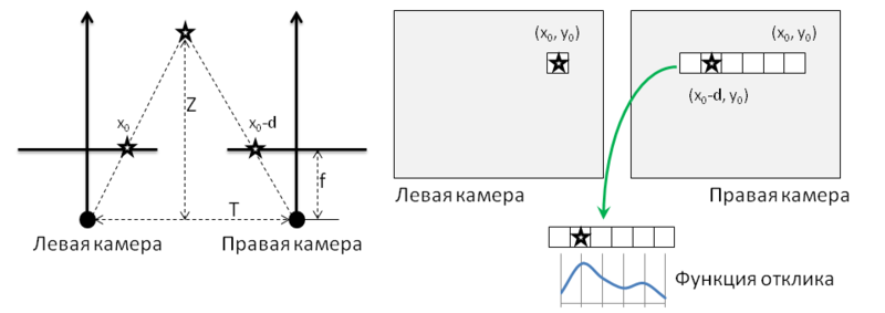
After the images are rectified, search for the corresponding pairs of points. The simplest method is illustrated in Figure 4 and consists of the following. For each pixel of the left image with coordinates ( x 0 , y 0 ), a pixel search is performed on the right image. It is assumed that the pixel in the right picture should have coordinates ( x 0 - d , y 0 ), where d- a value called a disparity. The search for the corresponding pixel is performed by calculating the maximum of the response function, which, for example, can be the correlation of pixel neighborhoods. The result is a disparity map, an example of which is shown in Fig. 3.
Figure 3: An example of rectified images, and their corresponding disparity map.


The actual depth values are inversely proportional to the magnitude of the pixel displacement. If we use the notation on the left half of Figure 4, then the relationship between disparity and depth can be expressed in the following way:
Figure 4: Computing a depth map.
Due to the inverse relationship of depth and displacement, the resolution of stereo vision systems that operate on the basis of this method is better at short distances, and worse at far distances.