Introduction to Machine Learning
- Tutorial
The full course in Russian can be found at this link .
The original English course is available at this link .

New lectures are scheduled every 2-3 days.
“Hello again, I’m Paige and you are my guest today, Sebastian.”
- Hi, I'm Sebastian!
- ... a man who has an incredible career, who managed to do a lot of amazing things! You are a co-founder of Udacity, you founded Google X, you are a professor at Stanford. You have been doing incredible research and deep learning throughout your career. What brought you the most satisfaction and in which of the areas did you receive the most rewards for the work done?
- Frankly, I really love being in Silicon Valley! I like to be near people who are much smarter than me, and I always considered technology as a tool that changes the rules of the game in various ways - from education to logistics, healthcare, etc. All this changes so quickly, and there is an incredible desire to be a participant in these changes, to observe them. You look at your surroundings and understand that most of what you see around you does not work as it should - you can always invent something new!
- Well, this is a very optimistic view of technology! What was the biggest eureka throughout your career?
- Lord, there were so many! I remember one of the days when Larry Page called me and suggested creating autopilot cars that could drive through all the streets of California. At that time I was considered an expert, I was ranked among those and, I was the very person who said "no, this cannot be done." After that, Larry convinced me that, in principle, it is possible to do this, you just have to start and try. And we did it! This was the moment when I realized that even experts are wrong and saying “no” we are 100% pessimistic. I think we should be more open to the new.
- Or, for example, if Larry Page calls you and says, “Hey, do a cool thing like Google X” and you get something pretty cool!
- Yes, that's for sure, no need to complain! I mean, all this is a process that goes through a lot of discussion on the way to implementation. I am really lucky to work and I'm proud of it, on Google X and on other projects.
- Awesome! So, this course is all about working with TensorFlow. Do you have experience using TensorFlow or maybe you are familiar (heard) with it?
- Yes! I literally love TensorFlow, of course! In my own laboratory, we use it often and a lot, one of the most significant works based on TensorFlow was released about two years ago. We learned that iPhone and Android can be more effective at detecting skin cancer than the best dermatologists in the world. We published our research in Nature and this created a kind of commotion in medicine.
- That sounds amazing! So you know and love TensorFlow, which is great in itself! Have you already worked with TensorFlow 2.0?
- No, unfortunately I have not had time yet.
- He will be just amazing! All students in this course will work with this version.
- I envy them! I will definitely try it!
- Perfectly! In our course there are a lot of students who in their life have never been engaged in machine learning, from the word "completely". For them, the field may be new, perhaps for someone programming itself will be new. What advice do you have for them?
- I would wish them to remain open - to new ideas, techniques, solutions, positions. Machine learning is actually easier than programming. In the programming process, you need to take into account each case in the source data, adapt the program logic and rules for it. At this very time, using TensorFlow and machine learning, you essentially train the computer using examples, letting the computer find the rules itself.
- This is incredibly interesting! I can't wait to tell students in this course a little more about machine learning! Sebastian, thank you for taking the time to come to us today!
- Thank you! Stay in touch!
So, let's start with the following task - given input and output values.

When you have the value 0 as the input value, then 32 as the output value. When you have 8 as the input value, then 46.4 as the output value. When you have 15 as the input value, then 59 as the output value, and so on.
Take a closer look at these values and let me ask you a question. Can you determine what the output will be if we get 38 at the input?

If you answered 100.4, then you were right!

So, how could we solve this problem? If you look closely at the values, you can see that they are related by the expression:

Where C - degrees Celsius (input values), F - Fahrenheit (output values).
What your brain has just done - compared input values and output values and found a common model (connection, dependence) between them - this is what machine learning does.
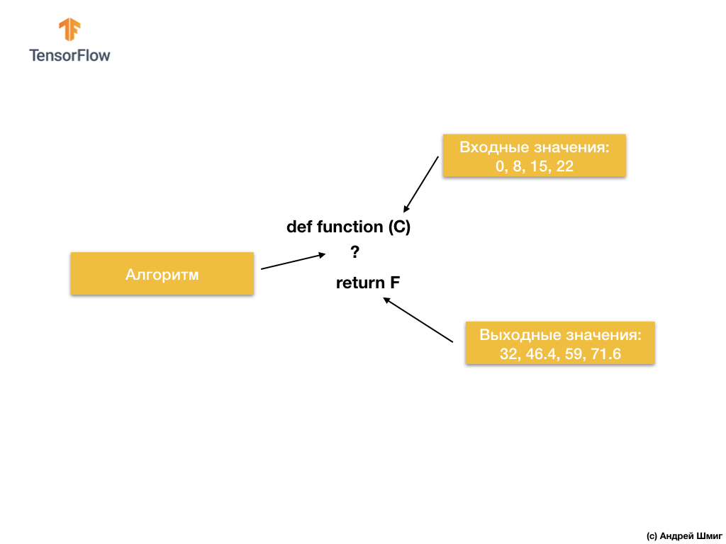
Based on the input and output values, machine learning algorithms will find a suitable algorithm for converting input values to output ones. This can be represented as follows:

Let's look at an example. Imagine that we want to develop a program that will convert degrees Celsius to degrees Fahrenheit using the formula

The solution, when approaching from the point of view of traditional software development, can be implemented in any programming language using the function:

So what do we have? The function takes an input value of C, then calculates the output value of F using an explicit algorithm, and then returns the calculated value.

On the other hand, in the machine learning approach, we only have input and output values, but not the algorithm itself:
The machine learning approach is based on using neural networks to find the relationship between input and output values.

You can think of neural networks as a stack of layers, each of which consists of previously known mathematics (formulas) and internal variables. The input value enters the neural network and passes through a stack of layers of neurons. While passing through the layers, the input value is converted according to the mathematics (given formulas) and the values of the internal variables of the layers, producing an output value.
In order for the neural network to be able to learn and determine the correct relationship between the input and output values, we need to train it - to train.
We train the neural network through repeated attempts to match input values to output ones.

In the process of training, the “fitting” (selection) of the values of internal variables in the layers of the neural network takes place until the network learns to generate the corresponding output values to the corresponding input values.
As we will see later, in order to train a neural network and allow it to select the most suitable values of internal variables, thousands or tens of thousands of iterations (trainings) are performed.

As a simplified version of understanding machine learning, you can imagine machine learning algorithms as functions that select the values of internal variables so that the correct input values correspond to the correct output values.
There are many types of neural network architectures. However, no matter what architecture you choose, the math inside (which calculations are performed and in what order) will remain unchanged during the training. Instead of changing maths, internal variables (weights and offsets) change during training.
For example, in the task of converting from degrees Celsius to Fahrenheit, the model starts by multiplying the input value by a certain number (weight) and adding another value (offset). Model training consists in finding suitable values for these variables, without changing the performed operations of multiplication and addition.
But one cool thing to think about! If you solved the problem of converting degrees Celsius to Fahrenheit, which is indicated in the video and in the text below, you probably solved it because you had some previous experience or knowledge on how to perform this kind of conversion from degrees Celsius to Fahrenheit. For example, you might just know that 0 degrees Celsius corresponds to 32 degrees Fahrenheit. On the other hand, systems based on machine learning do not have previous supporting knowledge to solve the problem. They learn to solve such problems not based on previous knowledge and in their complete absence.
Enough talk - move on to the practical part of the lecture!
The Russian version of CoLab source code and the English version of CoLab source code .
Welcome to CoLab, where we will train our first machine learning model!
We will try to maintain the simplicity of the material presented and introduce only the basic concepts necessary for the work. Subsequent CoLabs will contain more advanced techniques.
The task that we will solve is the conversion of degrees Celsius to degrees Fahrenheit. The conversion formula is as follows:
Of course, it would be easier just to write a conversion function in Python or any other programming language that would perform direct calculations, but in this case it would not be machine learning :)
Instead, we will provide the TensorFlow input with our input values of degrees Celsius ( 0, 8, 15, 22, 38) and their respective degrees Fahrenheit (32, 46, 59, 72, 100). Then we will train the model in such a way that it approximately corresponds to the above formula.
The first thing we import
Next, import
As we saw earlier, the machine learning technique with the teacher is based on the search for an algorithm for converting input data to output. Since the goal of this CoLab is to create a model that can produce the result of converting degrees Celsius to degrees Fahrenheit, we will create two lists -
Some machine learning terminology:
Next we create a model. We will use the most simplified model - the model of a fully connected network (
We will name the layer
Once layers are defined they need to be converted to a model.
Our model has only one layer -
Note
Quite often, you will encounter the definition of layers directly in the model function, rather than their preliminary description and subsequent use:
Before training, the model must be compiled (assembled). When compiling for training, you need:
The loss function and optimization function are used during model training (
The action of calculating the current losses and the subsequent improvement of these values in the model is exactly what training is (one iteration).
During training, the optimization function is used to calculate adjustments to the values of internal variables. The goal is to adjust the values of internal variables in such a way in the model (and this, in fact, is a mathematical function) so that they reflect as closely as possible the existing expression for converting degrees Celsius to degrees Fahrenheit.
TensorFlow uses numerical analysis to perform these kinds of optimization operations, and all this complexity is hidden from our eyes, so we will not go into details in this course.
What is useful to know about these parameters:
The loss function (standard error) and the optimization function (Adam) used in this example are standard for such simple models, but many others are available besides them. At this stage, we don’t care how these functions work.
What you should pay attention to is the optimization function and the parameter is the learning rate coefficient (
Training of the model is carried out by the method
During training, the model receives degrees Celsius at the input, performs transformations using the values of internal variables (called “weights”) and returns values that must correspond to degrees Fahrenheit. Since the initial values of the weights are set arbitrarily, the resulting values will be far from the correct values. The difference between the desired result and the actual is calculated using the loss function, and the optimization function determines how weights should be adjusted.
This cycle of calculations, comparisons and adjustments is controlled within the method
In the following videos, we will dive into the details of how this all works and how exactly the fully-connected layers (
The method
We will use for visualization

Now we have a model that has been trained on input values
For example, how much is 100.0 degrees Celsius Fahrenheit? Try to guess before you run the code below.
Conclusion: The correct answer is 100 × 1.8 + 32 = 212, so our model did pretty well! Review
Our model fitted the values of the internal variables (weights) into a
Let's display the values of the internal variables of the
Conclusion:
The value of the first variable is close to ~ 1.8, and the second to ~ 32. These values (1.8 and 32) are direct values in the formula for converting degrees Celsius to degrees Fahrenheit.
This is really very close to the actual values in the formula! We will consider this point in more detail in subsequent videos, where we show how the-
Since the representations are the same, the values of the internal variables of the model should converge to those presented in the actual formula, which happened in the end.
With the presence of additional neurons, additional input values and output values, the formula becomes a little more complicated, but the essence remains the same.
For fun! What happens if we create more
Conclusion:
As you may have noticed, the current model is also capable of predicting quite well the corresponding degrees of Fahrenheit. However, if we look at the values of the internal variables (weights) of neurons by layers, then we will not see any values similar to 1.8 and 32. The added complexity of the model hides the “simple” form of converting degrees Celsius to degrees Fahrenheit.
Stay connected and in the next part we will look at how Dense layers work “under the hood”.
Congratulations! You have just trained your first model. In practice, we saw how, by input and output values, the model learned to multiply the input value by 1.8 and add 32 to it to get the correct result.

This was really impressive, considering how many lines of code we needed to write:
The above example is a general plan for all machine learning programs. You will use similar constructions to create and train neural networks and to solve subsequent problems.
The training process (taking place in the method
In order to engage in machine learning, you, in principle, do not need to understand these details. But for those who are still interested in learning more: gradient descent through iterations changes the parameter values a little bit, “pulling” them in the right direction, until the best results are obtained. In this case, “best results” (best values) mean that any subsequent change in the parameter will only worsen the result of the model. A function that measures how good or bad a model is at each iteration is called a “loss function”, and the goal of each “pull” (adjustment of internal values) is to reduce the value of the loss function.
The training process begins with the “direct distribution” block, in which the input parameters go to the input of the neural network, follow the hidden neurons and then go to the weekend. The model then applies internal transformations on the input values and internal variables to predict the response.
In our example, the input value is the temperature in degrees Celsius and the model predicted the corresponding value in degrees Fahrenheit.

As soon as the value is predicted, the difference between the predicted value and the correct one is calculated. The difference is called “loss” and is a form of measurement of how well the model worked. The loss value is calculated by the loss function, which we determined by one of the arguments when calling the method
After calculating the loss value, the internal variables (weights and displacements) of all layers of the neural network are adjusted to minimize the loss value in order to approximate the output value to the correct initial reference value.

This optimization process is called gradient descent . A specific optimization algorithm is used to calculate a new value for each internal variable when the method is called
Understanding the principles of the training process is not required for this course, however if you are curious enough you can find more information on the Google Crash Course(The translation and the practical part of the entire course are laid down in the author's plans for publication).
By this point, you should already be familiar with the following terms:
In the previous part, we created a model that converts degrees Celsius to degrees Fahrenheit using a simple neural network to find the relationship between degrees Celsius and degrees Fahrenheit.
Our network consists of a single fully connected layer. But what is a fully connected layer? To figure this out, let's create a more complex neural network with 3 input parameters, one hidden layer with two neurons and one output layer with a single neuron.

Recall that a neural network can be imagined as a set of layers, each of which consists of nodes called neurons. Neurons at each level can be connected to the neurons of each subsequent layer. The type of layers in which each neuron of one layer is connected to each other neuron of the next layer is called a fully connected (fully connected) or dense layer (

Thus, when we use fully connected layers in
To create the above neural network, the following expressions are enough for us:
So, we figured out what neurons are and how they are related. But how do fully connected layers actually work?
To understand what is really happening there and what they are doing, we need to look “under the hood” and take apart the internal mathematics of neurons.

Imagine that our model receives three parameters -

What you should definitely keep in mind is that the internal mathematics of the neuron remains unchanged . In other words, during the training process, only weights and displacements change .
When you start learning machine learning, it may seem strange - the fact that it really works, but that is how machine learning works!
Let's get back to our example of converting degrees Celsius to degrees Fahrenheit.

With a single neuron, we have only one weight and one displacement. You know what? This is exactly what the formula for converting degrees Celsius to degrees Fahrenheit looks like. If we substitute the
If we return to the results of our model from the practical part, we will pay attention to the fact that the indicators of weight and displacement were “calibrated” in such a way that approximately correspond to the values from the formula.
We purposefully created just such a practical example in order to clearly show the exact comparison between weights and offsets. Putting machine learning into practice, we can never compare the values of variables with the target algorithm in this way, as in the example above. How can we do this? No way, because we don’t even know the target algorithm!
Solving the problems of machine learning, we test various architectures of neural networks with a different number of neurons in them - by trial and error we find the most accurate architectures and models and hope that they will solve the task in the learning process. In the next practical part, we will be able to study specific examples of this approach.
Stay in touch, because now the fun begins!
In this lesson we learned basic approaches in machine learning and learned how fully connected layers (
... and standard call-to-action - sign up, put a plus and do share :)
YouTube: https://youtube.com/channel/ashmig
Telegram: https://t.me/ashmig
VK: https://vk.com/ashmig
The original English course is available at this link .
New lectures are scheduled every 2-3 days.
Interview with Sebastian Trun, CEO Udacity
“Hello again, I’m Paige and you are my guest today, Sebastian.”
- Hi, I'm Sebastian!
- ... a man who has an incredible career, who managed to do a lot of amazing things! You are a co-founder of Udacity, you founded Google X, you are a professor at Stanford. You have been doing incredible research and deep learning throughout your career. What brought you the most satisfaction and in which of the areas did you receive the most rewards for the work done?
- Frankly, I really love being in Silicon Valley! I like to be near people who are much smarter than me, and I always considered technology as a tool that changes the rules of the game in various ways - from education to logistics, healthcare, etc. All this changes so quickly, and there is an incredible desire to be a participant in these changes, to observe them. You look at your surroundings and understand that most of what you see around you does not work as it should - you can always invent something new!
- Well, this is a very optimistic view of technology! What was the biggest eureka throughout your career?
- Lord, there were so many! I remember one of the days when Larry Page called me and suggested creating autopilot cars that could drive through all the streets of California. At that time I was considered an expert, I was ranked among those and, I was the very person who said "no, this cannot be done." After that, Larry convinced me that, in principle, it is possible to do this, you just have to start and try. And we did it! This was the moment when I realized that even experts are wrong and saying “no” we are 100% pessimistic. I think we should be more open to the new.
- Or, for example, if Larry Page calls you and says, “Hey, do a cool thing like Google X” and you get something pretty cool!
- Yes, that's for sure, no need to complain! I mean, all this is a process that goes through a lot of discussion on the way to implementation. I am really lucky to work and I'm proud of it, on Google X and on other projects.
- Awesome! So, this course is all about working with TensorFlow. Do you have experience using TensorFlow or maybe you are familiar (heard) with it?
- Yes! I literally love TensorFlow, of course! In my own laboratory, we use it often and a lot, one of the most significant works based on TensorFlow was released about two years ago. We learned that iPhone and Android can be more effective at detecting skin cancer than the best dermatologists in the world. We published our research in Nature and this created a kind of commotion in medicine.
- That sounds amazing! So you know and love TensorFlow, which is great in itself! Have you already worked with TensorFlow 2.0?
- No, unfortunately I have not had time yet.
- He will be just amazing! All students in this course will work with this version.
- I envy them! I will definitely try it!
- Perfectly! In our course there are a lot of students who in their life have never been engaged in machine learning, from the word "completely". For them, the field may be new, perhaps for someone programming itself will be new. What advice do you have for them?
- I would wish them to remain open - to new ideas, techniques, solutions, positions. Machine learning is actually easier than programming. In the programming process, you need to take into account each case in the source data, adapt the program logic and rules for it. At this very time, using TensorFlow and machine learning, you essentially train the computer using examples, letting the computer find the rules itself.
- This is incredibly interesting! I can't wait to tell students in this course a little more about machine learning! Sebastian, thank you for taking the time to come to us today!
- Thank you! Stay in touch!
What is machine learning?
So, let's start with the following task - given input and output values.
When you have the value 0 as the input value, then 32 as the output value. When you have 8 as the input value, then 46.4 as the output value. When you have 15 as the input value, then 59 as the output value, and so on.
Take a closer look at these values and let me ask you a question. Can you determine what the output will be if we get 38 at the input?
If you answered 100.4, then you were right!
So, how could we solve this problem? If you look closely at the values, you can see that they are related by the expression:
Where C - degrees Celsius (input values), F - Fahrenheit (output values).
What your brain has just done - compared input values and output values and found a common model (connection, dependence) between them - this is what machine learning does.
Based on the input and output values, machine learning algorithms will find a suitable algorithm for converting input values to output ones. This can be represented as follows:
Let's look at an example. Imagine that we want to develop a program that will convert degrees Celsius to degrees Fahrenheit using the formula
F = C * 1.8 + 32. The solution, when approaching from the point of view of traditional software development, can be implemented in any programming language using the function:
So what do we have? The function takes an input value of C, then calculates the output value of F using an explicit algorithm, and then returns the calculated value.
On the other hand, in the machine learning approach, we only have input and output values, but not the algorithm itself:
The machine learning approach is based on using neural networks to find the relationship between input and output values.
You can think of neural networks as a stack of layers, each of which consists of previously known mathematics (formulas) and internal variables. The input value enters the neural network and passes through a stack of layers of neurons. While passing through the layers, the input value is converted according to the mathematics (given formulas) and the values of the internal variables of the layers, producing an output value.
In order for the neural network to be able to learn and determine the correct relationship between the input and output values, we need to train it - to train.
We train the neural network through repeated attempts to match input values to output ones.
In the process of training, the “fitting” (selection) of the values of internal variables in the layers of the neural network takes place until the network learns to generate the corresponding output values to the corresponding input values.
As we will see later, in order to train a neural network and allow it to select the most suitable values of internal variables, thousands or tens of thousands of iterations (trainings) are performed.
As a simplified version of understanding machine learning, you can imagine machine learning algorithms as functions that select the values of internal variables so that the correct input values correspond to the correct output values.
There are many types of neural network architectures. However, no matter what architecture you choose, the math inside (which calculations are performed and in what order) will remain unchanged during the training. Instead of changing maths, internal variables (weights and offsets) change during training.
For example, in the task of converting from degrees Celsius to Fahrenheit, the model starts by multiplying the input value by a certain number (weight) and adding another value (offset). Model training consists in finding suitable values for these variables, without changing the performed operations of multiplication and addition.
But one cool thing to think about! If you solved the problem of converting degrees Celsius to Fahrenheit, which is indicated in the video and in the text below, you probably solved it because you had some previous experience or knowledge on how to perform this kind of conversion from degrees Celsius to Fahrenheit. For example, you might just know that 0 degrees Celsius corresponds to 32 degrees Fahrenheit. On the other hand, systems based on machine learning do not have previous supporting knowledge to solve the problem. They learn to solve such problems not based on previous knowledge and in their complete absence.
Enough talk - move on to the practical part of the lecture!
CoLab: convert degrees Celsius to degrees Fahrenheit
The Russian version of CoLab source code and the English version of CoLab source code .
The basics: learning the first model
Welcome to CoLab, where we will train our first machine learning model!
We will try to maintain the simplicity of the material presented and introduce only the basic concepts necessary for the work. Subsequent CoLabs will contain more advanced techniques.
The task that we will solve is the conversion of degrees Celsius to degrees Fahrenheit. The conversion formula is as follows:

Of course, it would be easier just to write a conversion function in Python or any other programming language that would perform direct calculations, but in this case it would not be machine learning :)
Instead, we will provide the TensorFlow input with our input values of degrees Celsius ( 0, 8, 15, 22, 38) and their respective degrees Fahrenheit (32, 46, 59, 72, 100). Then we will train the model in such a way that it approximately corresponds to the above formula.
Import Dependencies
The first thing we import
TensorFlow. Hereinafter, we abbreviated it tf. We also configure the level of logging - only errors. Next, import
NumPyas np. NumpyHelps us present our data as high-performance listings.from __future__ import absolute_import, division, print_function, unicode_literals
import tensorflow as tf
tf.logging.set_verbosity(tf.logging.ERROR)
import numpy as np
Training data preparation
As we saw earlier, the machine learning technique with the teacher is based on the search for an algorithm for converting input data to output. Since the goal of this CoLab is to create a model that can produce the result of converting degrees Celsius to degrees Fahrenheit, we will create two lists -
celsius_qand fahrenheit_awhich we use when training our model.celsius_q = np.array([-40, -10, 0, 8, 15, 22, 38], dtype=float)
fahrenheit_a = np.array([-40, 14, 32, 46, 59, 72, 100], dtype=float)
for i,c in enumerate(celsius_q):
print("{} градусов Цельсия = {} градусов Фаренгейта".format(c, fahrenheit_a[i]))
-40.0 градусов Цельсия = -40.0 градусов Фаренгейта

-10.0 градусов Цельсия = 14.0 градусов Фаренгейта

0.0 градусов Цельсия = 32.0 градусов Фаренгейта

8.0 градусов Цельсия = 46.0 градусов Фаренгейта

15.0 градусов Цельсия = 59.0 градусов Фаренгейта

22.0 градусов Цельсия = 72.0 градусов Фаренгейта

38.0 градусов Цельсия = 100.0 градусов Фаренгейта
Some machine learning terminology:
- Property is the input value (s) of our model. In this case, the unit value is degrees Celsius.
- Labels are the output values that our model predicts. In this case, the unit value is degrees Fahrenheit.
- An example is a pair of input-output values used for training. In this case, it is a pair of values from
celsius_qandfahrenheit_aunder a certain index, for example, (22,72).
Create a model
Next we create a model. We will use the most simplified model - the model of a fully connected network (
Dense-network). Since the task is quite trivial, the network will also consist of a single layer with a single neuron.Building a network
We will name the layer
l0( l ayer and zero) and create it by initializing tf.keras.layers.Densewith the following parameters:input_shape=[1]- this parameter determines the dimension of the input parameter - a single value. 1 × 1 matrix with a single value. Since this is the first (and only) layer, the dimension of the input data corresponds to the dimension of the entire model. The only value is a floating point value representing degrees Celsius.units=1- This parameter determines the number of neurons in the layer. The number of neurons determines how many internal layer variables will be used for training in finding a solution to the problem. Since this is the last layer, its dimension is equal to the dimension of the result - the output value of the model - a single floating-point number representing degrees Fahrenheit. (In a multilayer network, the size and shape of the layerinput_shapemust correspond to the size and shape of the next layer).
l0 = tf.keras.layers.Dense(units=1, input_shape=[1])
Convert layers to model
Once layers are defined they need to be converted to a model.
Sequential-model takes as arguments the list of layers in the order in which they must be applied - from the input value to the output value. Our model has only one layer -
l0.model = tf.keras.Sequential([l0])
Note
Quite often, you will encounter the definition of layers directly in the model function, rather than their preliminary description and subsequent use:
model = tf.keras.Sequential([
    tf.keras.layers.Dense(units=1, input_shape=[1])
])
We compile a model with a loss and optimization function
Before training, the model must be compiled (assembled). When compiling for training, you need:
- loss function - a way of measuring how far the predicted value is from the desired output value (a measurable difference is called “loss”).
- optimization function - a way to adjust internal variables to reduce losses.
model.compile(loss='mean_squared_error',
              optimizer=tf.keras.optimizers.Adam(0.1))
The loss function and optimization function are used during model training (
model.fit(...)mentioned below) to perform initial calculations at each point and then optimize the values. The action of calculating the current losses and the subsequent improvement of these values in the model is exactly what training is (one iteration).
During training, the optimization function is used to calculate adjustments to the values of internal variables. The goal is to adjust the values of internal variables in such a way in the model (and this, in fact, is a mathematical function) so that they reflect as closely as possible the existing expression for converting degrees Celsius to degrees Fahrenheit.
TensorFlow uses numerical analysis to perform these kinds of optimization operations, and all this complexity is hidden from our eyes, so we will not go into details in this course.
What is useful to know about these parameters:
The loss function (standard error) and the optimization function (Adam) used in this example are standard for such simple models, but many others are available besides them. At this stage, we don’t care how these functions work.
What you should pay attention to is the optimization function and the parameter is the learning rate coefficient (
learning rate), which in our example is0.1. This is the used step size when adjusting the internal values of variables. If the value is too small, it will take too many training iterations to train the model. Too much - accuracy drops. Finding a good value for the coefficient of learning speed requires some trial and error, it usually ranges from 0.01(by default) to 0.1.We train the model
Training of the model is carried out by the method
fit. During training, the model receives degrees Celsius at the input, performs transformations using the values of internal variables (called “weights”) and returns values that must correspond to degrees Fahrenheit. Since the initial values of the weights are set arbitrarily, the resulting values will be far from the correct values. The difference between the desired result and the actual is calculated using the loss function, and the optimization function determines how weights should be adjusted.
This cycle of calculations, comparisons and adjustments is controlled within the method
fit. The first argument is the input value, the second argument is the desired output value. Argumentepochsdetermines how many times this training cycle should be completed. The argument verbosecontrols the level of logging.history = model.fit(celsius_q, fahrenheit_a, epochs=500, verbose=False)
print("Завершили тренировку модели")
In the following videos, we will dive into the details of how this all works and how exactly the fully-connected layers (
Denselayers) work “under the hood”.Display training statistics
The method
fitreturns an object that contains information about the change in losses with each subsequent iteration. We can use this object to build an appropriate loss schedule. High loss means that the Fahrenheit degrees predicted by the model are far from the true values in the array fahrenheit_a. We will use for visualization
Matplotlib. As you can see, our model improves very quickly at the very beginning, and then comes to a stable and slow improvement until the results become “near” -perfect at the very end of the training.import matplotlib.pyplot as plt
plt.xlabel('Epoch')
plt.ylabel('Loss')
plt.plot(history.history['loss'])
We use the model for predictions.
Now we have a model that has been trained on input values
celsius_qand output values fahrenheit_ato determine the relationship between them. We can use the prediction method to calculate the Fahrenheit degrees by which we previously did not know the corresponding degrees Celsius. For example, how much is 100.0 degrees Celsius Fahrenheit? Try to guess before you run the code below.
print(model.predict([100.0]))
Conclusion: The correct answer is 100 × 1.8 + 32 = 212, so our model did pretty well! Review
[[211.29639]]
- We created a model using the
Dense-layer - We trained her with 3,500 examples (7 pairs of values, 500 training iterations)
Our model fitted the values of the internal variables (weights) into a
Denselayer in such a way as to return the correct values of degrees Fahrenheit to an arbitrary input value of degrees Celsius.We look at the weights
Let's display the values of the internal variables of the
Dense-layer.print("Это значения переменных слоя: {}".format(l0.get_weights()))
Conclusion:
Это значения переменных слоя: [array([[1.8261501]], dtype=float32), array([28.681389], dtype=float32)]
The value of the first variable is close to ~ 1.8, and the second to ~ 32. These values (1.8 and 32) are direct values in the formula for converting degrees Celsius to degrees Fahrenheit.
This is really very close to the actual values in the formula! We will consider this point in more detail in subsequent videos, where we show how the-
Denselayer works , but for now it’s worth knowing only that one neuron with a single input and output contains simple mathematics - y = mx + b(as an equation of a line), which is nothing but our formula for converting degrees Celsius to degrees Fahrenheit f = 1.8c + 32. Since the representations are the same, the values of the internal variables of the model should converge to those presented in the actual formula, which happened in the end.
With the presence of additional neurons, additional input values and output values, the formula becomes a little more complicated, but the essence remains the same.
A bit of experimentation
For fun! What happens if we create more
Denseβ-layers with more neurons, which in turn will contain more internal variables?l0 = tf.keras.layers.Dense(units=4, input_shape=[1])
l1 = tf.keras.layers.Dense(units=4)
l2 = tf.keras.layers.Dense(units=1)
model = tf.keras.Sequential([l0, l1, l2])
model.compile(loss='mean_squared_error', optimizer=tf.keras.optimizers.Adam(0.1))
model.fit(celsius_q, fahrenheit_a, epochs=500, verbose=False)
print("Закончили обучение модели")
print(model.predict([100.0]))
print("Модель предсказала, что 100 градусов Цельсия соответствуют {} градусам Фаренгейта".format(model.predict([100.0])))
print("Значения внутренних переменных слоя l0: {}".format(l0.get_weights()))
print("Значения внутренних переменных слоя l1: {}".format(l1.get_weights()))
print("Значения внутренних переменных слоя l2: {}".format(l2.get_weights()))
Conclusion:
Закончили обучение модели
[[211.74748]]
Модель предсказала, что 100 градусов Цельсия соответствуют [[211.74748]] градусам Фаренгейта
Значения внутренних переменных слоя l0: [array([[-0.5972079 , -0.05531882, -0.00833384, -0.10636603]],
      dtype=float32), array([-3.0981746, -1.8776944,  2.4708805, -2.9092448], dtype=float32)]
Значения внутренних переменных слоя l1: [array([[ 0.09127654,  1.1659832 , -0.61909443,  0.3422218 ],
       [-0.7377194 ,  0.20082018, -0.47870865,  0.30302727],
       [-0.1370897 , -0.0667181 , -0.39285263, -1.1399261 ],
       [-0.1576551 ,  1.1161333 , -0.15552482,  0.39256814]],
      dtype=float32), array([-0.94946504, -2.9903848 ,  2.9848468 , -2.9061244 ], dtype=float32)]
Значения внутренних переменных слоя l2: [array([[-0.13567649],
       [-1.4634581 ],
       [ 0.68370366],
       [-1.2069695 ]], dtype=float32), array([2.9170544], dtype=float32)]
As you may have noticed, the current model is also capable of predicting quite well the corresponding degrees of Fahrenheit. However, if we look at the values of the internal variables (weights) of neurons by layers, then we will not see any values similar to 1.8 and 32. The added complexity of the model hides the “simple” form of converting degrees Celsius to degrees Fahrenheit.
Stay connected and in the next part we will look at how Dense layers work “under the hood”.
Brief Summary
Congratulations! You have just trained your first model. In practice, we saw how, by input and output values, the model learned to multiply the input value by 1.8 and add 32 to it to get the correct result.
This was really impressive, considering how many lines of code we needed to write:
l0 = tf.keras.layers.Dense(units=1, input_shape=[1])
model = tf.keras.Sequential([l0])
model.compile(loss='mean_squared_error', optimizer=tf.keras.optimizers.Adam(0.1))
history = model.fit(celsius_q, fahrenheit_a, epochs=500, verbose=False)
model.predict([100.0])
The above example is a general plan for all machine learning programs. You will use similar constructions to create and train neural networks and to solve subsequent problems.
Training process
The training process (taking place in the method
model.fit(...)) consists of a very simple sequence of actions, the result of which should be the values of internal variables giving the results as close as possible to the original. The optimization process by which such results are achieved, called gradient descent , uses numerical analysis to find the most suitable values for the internal variables of the model.In order to engage in machine learning, you, in principle, do not need to understand these details. But for those who are still interested in learning more: gradient descent through iterations changes the parameter values a little bit, “pulling” them in the right direction, until the best results are obtained. In this case, “best results” (best values) mean that any subsequent change in the parameter will only worsen the result of the model. A function that measures how good or bad a model is at each iteration is called a “loss function”, and the goal of each “pull” (adjustment of internal values) is to reduce the value of the loss function.
The training process begins with the “direct distribution” block, in which the input parameters go to the input of the neural network, follow the hidden neurons and then go to the weekend. The model then applies internal transformations on the input values and internal variables to predict the response.
In our example, the input value is the temperature in degrees Celsius and the model predicted the corresponding value in degrees Fahrenheit.
As soon as the value is predicted, the difference between the predicted value and the correct one is calculated. The difference is called “loss” and is a form of measurement of how well the model worked. The loss value is calculated by the loss function, which we determined by one of the arguments when calling the method
model.compile(...).After calculating the loss value, the internal variables (weights and displacements) of all layers of the neural network are adjusted to minimize the loss value in order to approximate the output value to the correct initial reference value.
This optimization process is called gradient descent . A specific optimization algorithm is used to calculate a new value for each internal variable when the method is called
model.compile(...). In the above example, we used an optimization algorithm Adam. Understanding the principles of the training process is not required for this course, however if you are curious enough you can find more information on the Google Crash Course(The translation and the practical part of the entire course are laid down in the author's plans for publication).
By this point, you should already be familiar with the following terms:
- Property : input value of our model;
- Examples : input + output pairs;
- Tags : model output values;
- Layers : a collection of nodes joined together within a neural network;
- Model : representation of your neural network;
- Dense and fully connected : each node in one layer is connected to each node from the previous layer.
- Weights and offsets : model internal variables;
- Loss : the difference between the desired output value and the actual output value of the model;
- MSE: среднеквадратичное отклонение, тип функции потерь, которые считают малое количество больших ошибок вариантом хуже, чем большое количество малых.
- Градиентный спуск: алгоритм, который изменяет внутренние переменные по-немногу при каждой итерации с целью уменьшения значения функции потерь;
- Оптимизатор: конкретная реализация алгоритма градиентного спуска;
- Коэффициент скорости обучения: размер «шага» при снижении потерь во время градиентного спуска;
- Серия: набор данных для обучения нейронной сети;
- Эпоха: полный проход по всей серии исходных данных;
- Прямое распространение: вычисление выходных значение по входным значениям;
- Back propagation : calculating the values of internal variables according to an optimization algorithm starting from the output layer and towards the input layer through all the intermediate layers.
Sense layers
In the previous part, we created a model that converts degrees Celsius to degrees Fahrenheit using a simple neural network to find the relationship between degrees Celsius and degrees Fahrenheit.
Our network consists of a single fully connected layer. But what is a fully connected layer? To figure this out, let's create a more complex neural network with 3 input parameters, one hidden layer with two neurons and one output layer with a single neuron.
Recall that a neural network can be imagined as a set of layers, each of which consists of nodes called neurons. Neurons at each level can be connected to the neurons of each subsequent layer. The type of layers in which each neuron of one layer is connected to each other neuron of the next layer is called a fully connected (fully connected) or dense layer (
Dense-layer). Thus, when we use fully connected layers in
keras, we kind of inform that the neurons of this layer should be connected to all the neurons of the previous layer. To create the above neural network, the following expressions are enough for us:
hidden = tf.keras.layers.Dense(units=2, input_shape=[3])
output = tf.keras.layers.Dense(units=1)
model = tf.keras.Sequential([hidden, output])
So, we figured out what neurons are and how they are related. But how do fully connected layers actually work?
To understand what is really happening there and what they are doing, we need to look “under the hood” and take apart the internal mathematics of neurons.
Imagine that our model receives three parameters -
х1, х2, х3, and а1, а2 и а3- the neurons of our network. Remember we said that a neuron has internal variables? So, w * and b * are the same internal variables of a neuron, also known as weights and displacements. It is the values of these variables that are adjusted in the learning process to obtain the most accurate results of comparing the input values to the output. What you should definitely keep in mind is that the internal mathematics of the neuron remains unchanged . In other words, during the training process, only weights and displacements change .
When you start learning machine learning, it may seem strange - the fact that it really works, but that is how machine learning works!
Let's get back to our example of converting degrees Celsius to degrees Fahrenheit.
With a single neuron, we have only one weight and one displacement. You know what? This is exactly what the formula for converting degrees Celsius to degrees Fahrenheit looks like. If we substitute the
w11value 1.8, and instead of b1- 32, we get the final transformation model! If we return to the results of our model from the practical part, we will pay attention to the fact that the indicators of weight and displacement were “calibrated” in such a way that approximately correspond to the values from the formula.
We purposefully created just such a practical example in order to clearly show the exact comparison between weights and offsets. Putting machine learning into practice, we can never compare the values of variables with the target algorithm in this way, as in the example above. How can we do this? No way, because we don’t even know the target algorithm!
Solving the problems of machine learning, we test various architectures of neural networks with a different number of neurons in them - by trial and error we find the most accurate architectures and models and hope that they will solve the task in the learning process. In the next practical part, we will be able to study specific examples of this approach.
Stay in touch, because now the fun begins!
Summary
In this lesson we learned basic approaches in machine learning and learned how fully connected layers (
Dense-layers) work. You trained your first model to convert degrees Celsius to degrees Fahrenheit. You also learned the basic terms used in machine learning, such as properties, examples, labels. You, among other things, wrote the main lines of code in Python, which are the backbone of any machine learning algorithm. You saw that in a few lines of code you can create, train and request a prediction from a neural network using TensorFlowand Keras. ... and standard call-to-action - sign up, put a plus and do share :)
Video version of the article
YouTube: https://youtube.com/channel/ashmig
Telegram: https://t.me/ashmig
VK: https://vk.com/ashmig