We work with neural networks: a checklist for debugging
- Transfer

Machine learning software code is often complex and rather confusing. Detecting and eliminating bugs in it is a resource-intensive task. Even the simplest direct-connected neural networks require a serious approach to network architecture, initialization of weights, and network optimization. A small mistake can lead to unpleasant problems.
This article is about the debugging algorithm of your neural networks.
Skillbox recommends: A hands-on course Python developer from scratch .
We remind you: for all readers of “Habr” - a discount of 10,000 rubles when registering for any Skillbox course using the “Habr” promo code.
The algorithm consists of five stages:
- simple start;
- confirmation of losses;
- verification of intermediate results and compounds;
- diagnostics of parameters;
- work control.
If something seems more interesting to you than the rest, you can go directly to these sections.
Easy start
A neural network with complex architecture, regularization, and a learning speed planner is harder to debut than a regular network. We are a little tricky here, since the item itself has an indirect relation to debugging, but this is still an important recommendation.
A simple start is to create a simplified model and train it on one data set (point).
First, create a simplified model.
For a quick start, create a small network with a single hidden layer and check that everything works correctly. Then we gradually complicate the model, checking every new aspect of its structure (additional layer, parameter, etc.), and move on.
We train the model on a single data set (point)
As a quick test of the health of your project, you can use one or two data points for training to confirm whether the system is working correctly. The neural network should show 100% accuracy of training and verification. If this is not the case, then either the model is too small or you already have a bug.
Even if all is well, prepare the model for the passage of one or more eras before moving on.
Loss estimate
Loss estimation is the main way to refine model performance. You need to make sure that the loss corresponds to the task, and the loss functions are evaluated on the correct scale. If you use more than one type of loss, then make sure that they are all of the same order and correctly scaled.
It is important to be attentive to the initial losses. Check how close the real result is to the expected if the model started with a random assumption. In the work of Andrei Karpati, the following is proposed.: “Make sure that you get the result expected when you start working with a small number of parameters. It is better to immediately check the data loss (with the degree of regularization set to zero). For example, for CIFAR-10 with the Softmax classifier, we expect the initial loss to be 2.302, because the expected diffuse probability is 0.1 for each class (since there are 10 classes), and the loss of Softmax is the negative logarithmic probability of the correct class as - ln (0.1) = 2.302. "
For a binary example, just a similar calculation is done for each of the classes. Here, for example, are the data: 20% 0's and 80% 1's. The expected initial loss will be up to –0.2ln (0.5) –0.8ln (0.5) = 0.693147. If the result is greater than 1, this may indicate that the weights of the neural network are not properly balanced or the data is not normalized.
Checking Intermediate Results and Connections
To debug a neural network, it is necessary to understand the dynamics of processes within the network and the role of individual intermediate layers, since they are connected. Here are some common mistakes you might encounter:
- Incorrect expressions for gradient updates
- weight updates do not apply;
- disappearing or exploding gradients.
If the gradient values are zero, this means that the learning speed in the optimizer is too slow, or that you encountered an incorrect expression to update the gradient.
In addition, it is necessary to monitor the values of the activation functions, weights and updates of each of the layers. For example, the value of parameter updates (weights and offsets) should be 1-e3 .
There is a phenomenon called the “Dying ReLU” or “Disappearing Gradient Problem,” when ReLU neurons will output zero after studying the large negative bias value for their weights. These neurons are never activated again in any data place.
You can use gradient testing to detect these errors by approximating the gradient using a numerical approach. If it is close to the calculated gradients, then back propagation was implemented correctly. To create a gradient test, check out these great resources from CS231 here and here , as well as a lesson Andrew Un (Andrew Nga) on this topic.
Fayzan Sheikh points out three main methods for visualizing a neural network:
- Preliminary - simple methods that show us the general structure of the trained model. They include the output of forms or filters of individual layers of the neural network and parameters in each layer.
- Based on activation. In them, we decipher the activation of individual neurons or groups of neurons in order to understand their functions.
- Gradient based. These methods tend to manipulate the gradients that form from the passage back and forth when training the model (including significance maps and class activation maps).
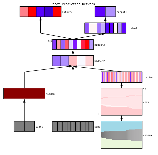
There are several useful tools for visualizing the activations and connections of individual layers, for example, ConX and Tensorboard .
Parameter Diagnostics
Neural networks have a lot of parameters that interact with each other, which complicates optimization. Actually, this section is the subject of active research by specialists, so the proposals below should be considered only as advice, the starting points from which you can build on.
Package size (batch size) - if you want the package size was large enough to produce accurate estimates of the gradient of the error, but small enough that the stochastic gradient descent (SGD) could organize your network. The small size of the packages will lead to a rapid convergence due to noise in the learning process and in the future - to the difficulties of optimization. This is described in more detail here .
Learning speed- too low will lead to slow convergence or the risk of being stuck in local lows. At the same time, a high learning speed will cause a discrepancy in optimization, since you risk "jumping" through the deep, but at the same time narrow part of the loss function. Try using speed planning to reduce it during neural network training. CS231n has a large section on this issue .
Gradient clipping - trimming the gradients of the parameters during back propagation at the maximum value or limit norm. Useful for solving problems with any exploding gradients that you may encounter in the third paragraph.
Batch normalization- used to normalize the input data of each layer, which allows to solve the problem of internal covariant shift. If you use Dropout and Batch Norma together, check out this article .
Stochastic Gradient Descent (SGD) - There are several varieties of SGD that use momentum, adaptive learning speeds, and the Nesterov method. At the same time, none of them has a clear advantage both in terms of learning efficiency and generalization ( details here ).
Regularization - is crucial for building a generalized model, because it adds a penalty for the complexity of the model or extreme parameter values. This is a way to reduce the dispersion of the model without significantly increasing its displacement. Moredetailed information is here .
In order to evaluate everything yourself, you need to disable regularization and check the gradient of data loss yourself.
Dropout is another way to streamline your network to prevent congestion. During training, loss occurs only by maintaining the activity of the neuron with a certain probability p (hyperparameter) or setting it to zero in the opposite case. As a result, the network must use a different subset of parameters for each training party, which reduces the changes in certain parameters that become dominant.
Important: if you use both dropout and batch normalization, be careful with the order of these operations or even with their joint use. All this is still being actively discussed and supplemented. Here are two important discussions on this topic on Stackoverflow and Arxiv .
Work control
It is about documenting workflows and experiments. If you don’t document anything, you can forget, for example, what kind of training speed or class weight is used. Thanks to the control, you can easily view and reproduce previous experiments. This reduces the number of duplicate experiments.
True, manual documentation can be challenging in the event of a large amount of work. This is where tools such as Comet.ml help you automatically log data sets, code changes, experiment history, and production models, including key information about your model (hyperparameters, model performance metrics, and environmental information).
A neural network can be very sensitive to small changes, and this will lead to a drop in model performance. Tracking and documenting work is the first step worth taking to standardize your environment and modeling.

I hope that this post can become the starting point from which you will begin debugging your neural network.
Skillbox recommends:
- Two-year practical course "I am a PRO web developer . "
- Online course "C # Developer with 0" .
- Practical annual course "PHP-developer from 0 to PRO" .